Week 2 - Flow over a Cylinder.
AIM:- The project aims to simulate the flow over a cylinder and explain the phenomenon of Karman vortex street.
OBJECTIVE OF THE PROJECT:- The objective is -
- Firstly, we discuss the phenomenon of Karman vortex street.
- The second objective is to simulate the flow with the steady and unsteady case and we also calculate the Strouhal Number for Re= 100.
- Then we calculate the coefficient of drag and lift over a cylinder by setting the Reynolds number to 10,100,1000,10000 & 100000.
- And we also discuss the effect of the Reynolds number on the coefficient of drag by comparing the results.
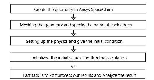
Workflow of the project and this is how the simulation we do.
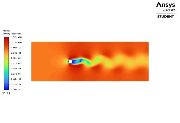
PROJECT DESCRIPTION:- External flow past around a circular cylinder has been extensively studied by the fluid community because of its practical applications. The flow of fluids over heat exchanger tubes and civil structures are such examples. The flow past a circular cylinder experiences a boundary layer separation and very strong flow oscillations in the region behind the body where recirculation happens. The flow pattern is dependent on the Reynold's number and is affected by factors such as surface roughness, the compressibility of the fluid, etc. In this project, we are going to simulate flow over a cylinder and understand how variations in the Reynold’s number impacts the recirculation that occurs behind the cylinder. In this simulation, we see how the vortices are created in the wake region of a cylinder.
In Fluid Mechanics, Vortex Shedding is a very important topic for Engineers. The vibrations generated by vortices near the body may cause the body to resonate to dangerous levels if the frequency of vortices is close to the natural frequency of the body – a situation that must be avoided in the design of equipment that is subjected to high-velocity fluid flow such as the wings of airplanes and suspended bridges subjected to steady high winds. Here our project is to simulate fluid flow over a cylinder and we know in the wake region the vortices are created because of flow separation and the Renolds number should be greater than 90. To dive into our project, first we discuss some terms which are associated with our project.
Karman Vortex Street:- In fluid dynamics, a Karman vortex street (or a von Kármán vortex street) is a repeating pattern of swirling vortices, caused by a process known as vortex shedding, which is responsible for the unsteady separation of flow of a fluid around blunt bodies.
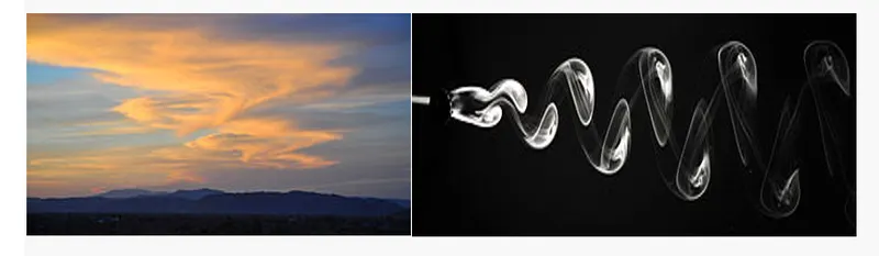
The first picture is a look at the Kármán vortex street effect from ground level, as air flows quickly from the pacific ocean eastward over Mojave desert mountains. This phenomenon observed from ground level is extremely rare, as most cloud-related Karman vortex street activity is viewed from space.
And the second picture is the visualization of the vortex street behind a circular cylinder in the air. The flow is made visible through the release of glycerol vapor in the air near the cylinder
Vortex shedding:- In fluid mechanics, an important consequence of flow separation is the formation and shedding of circulating fluid structures in the wake region is called Vortices. The periodic generation of these vortices downstream is reffered to as Vortex Shedding. In this flow, vortices are created at the back of the body and detach periodically from either side of the body forming a Von Karman vortex street. Vortex Shedding is not same as turbulent, we can see vortex shedding also in Laminar Flow.
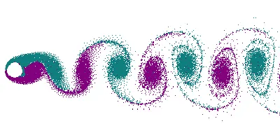
This is the animation of a vortex street created by a cylindrical object. The flow-on opposite sides of the object are given different colors that is showing the vortices are shed from alternating sides of the object
A vortex street will form only at a certain range of flow velocities, specified by a range of Reynold's number(Re). Typically above a limiting Reynolds number value of about 90. The Reynolds number for a flow is a measure of the ratio of inertial to viscous forces in the flow of a fluid around a body or a channel, and it may be defined as a nondimensional parameter of the global speed of the whole fluid flow:
`Re_L = (ρUL)/μ_0 = (UL)/nu_0`
Where, `Re_L` = Reynold's number,
`rho_0` = density of the fluid,
U = free stream velocity of the fluid,
L = Characteristic length of the body,
`mu_0` = The free stream Dynamic viscosity parameter of the fluid
`nu_0` = The free stream Kinematic viscosity parameter of the fluid and
`nu_0` = `mu_0/rho_0`
To know more about Vortex Shedding, we also have to know Strouhal number.
Strouhal Number:- Strouhal number is a dimensionless number which describes the oscillating flow mechanism. In a qualitative sense, it is the ratio of oscillation to mean speed.
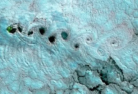
This is an alternating vortex in the clouds on the lee side of Tristan da Cunha, a volcanic island in the South Atlantic. The image was captured on June 25, 2017, by the Operational Land Imager on the Landsat 8 satellite. The image is false-color to better distinguish areas of land, water, and clouds. NASA Earth Observatory images by Joshua Stevens and Jesse Allen.
The formula of Strouhal number is -
`St = (f_w L)/U_∞`
where `f_w`is the frequency of the oscillations or vortex shedding frequency with dimensions [T-1], L is the characteristic length, and `U_∞` is the flow velocity. Best examples of such oscillations are found in vortex street wakes behind bluff bodies, as shown in the figure. The frequency of these oscillations can sometimes have a disastrous effect on the adjacent structures, as was the case in the collapse of the Tacoma Narrows Bridge in 1940 (Schagler, 1994).
Drag-Coefficient:-The force a flowing fluid exerts on a body in the flow direction is called Drag force. And the coefficient of drag is expressed as
`C_D = F_D/(1/2 rho V^2 A)`
Where, `F_D` is the lift force, `rho` is the density of fluid, V is the velocity of the fluid and A is taken to be planform area.
Lift-Coefficient:- Lift is difined as the component of net force (due to viscous and pressure forces) that is perpendicular to the flow direction, and the lift-coefficient is expressed as
`C_L = F_L/(1/2 rho V^2 A)`
Where, `F_L` is the lift force, `rho` is the density of fluid, V is the velocity of the fluid and A is taken to be planform area.
Now we can dive into our project. We divide our simulation in some part which we show in our workflow and we need to remember that our simulation is 2D.
GEOMETRY:-
First, we create our geometry in Ansys SpaceClaim. We first draw a cylinder whose diameter D is 2 meters. After that, we draw a construction line on the left side, which is 10D meters from the center of the cylinder, and on the right side, it is 20D meters from the center of the cylinder. And from the end side of the construction line, we draw an upper and lower line of 5D meters.
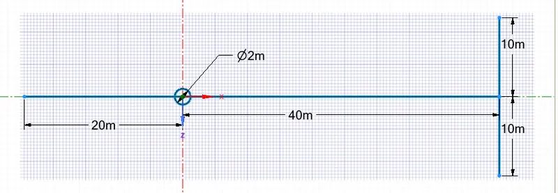
Then we draw a rectangle by using those edge points to create the boundary-
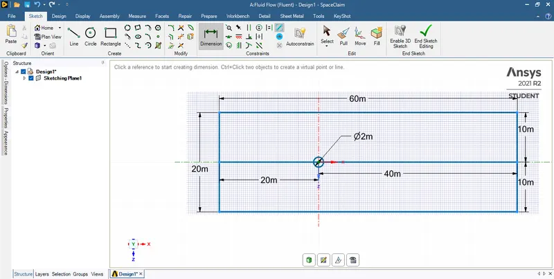
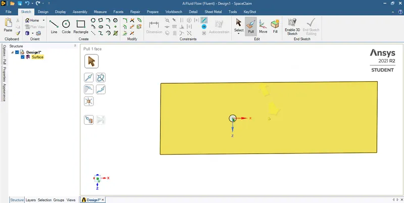
Then we delete the construction line and, for creating the surface, we are using the pull option in SpaceClaim –
Now, we delete the surface which is present in the cylinder. By using the select option, we select the cylindrical surface and delete it by pressing the delete key –
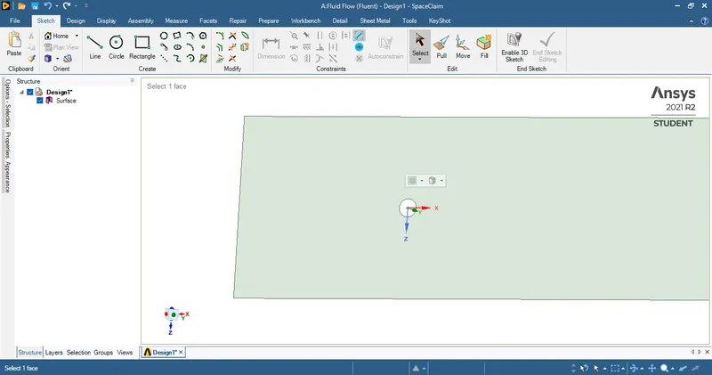
Now our geometry is complete
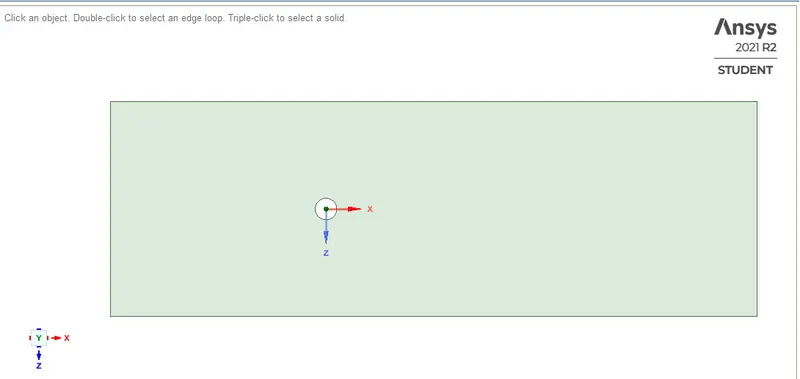
This is the last product which we should create for our simulation. Then we go for meshing.
MESHING AND NAMED SELECTION:- Now the meshing part is coming. Any continuous object has infinite degrees of freedom (DOF) which makes it impossible to solve using hand calculations. So we create a mesh that splits the domain into a discrete number of elements for which the solution can be calculated. The data is then interpolated across the whole domain. We first see the base meshing which is provided by Ansys by default.
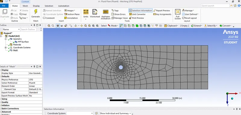
We can see that Ansys has done the fine mesh near the cylinder, and this is a very good feature provided by Ansys which automatically guess what portion needs more attention to simulate the model, but we need more refined mesh near the cylinder and also the whole geometry for the simulation. First, I give the size of 0.5m and click on generate mesh option. After that, We select the triangle method. To do that first we insert the Method option
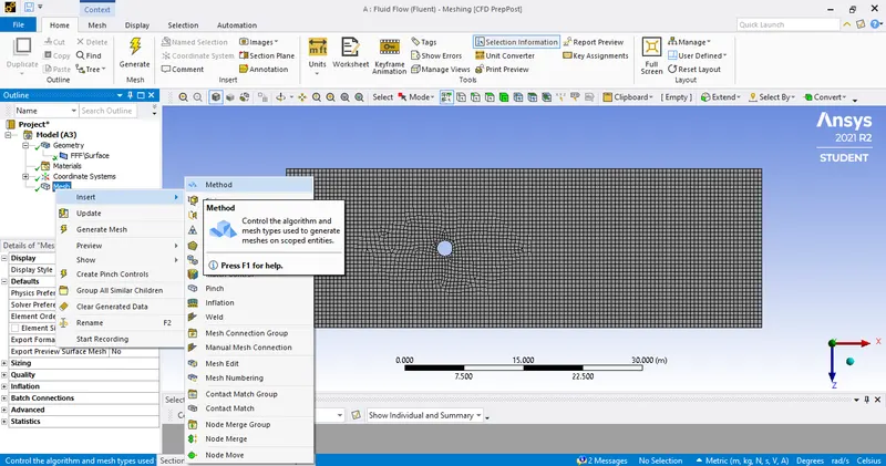
and then select the geometry and then we select triangules method. First, the method is Quadrilateral, and now triangles
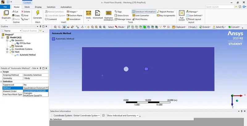
And now we click on Generate mesh option-
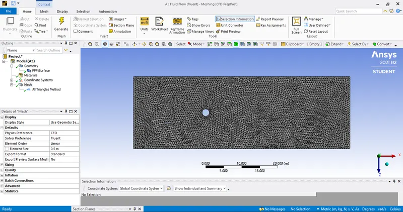
Now, if we see the circle very closely then we find that the circle is more like a polygon and we also know that we never get a perfect circle unless we do an infinite number of cells. But here we see some sharp corners which can affect the flow field. Since the cylinder on the top of which we are trying to simulate the flow, we have to make sure that the results are captured perfectly.
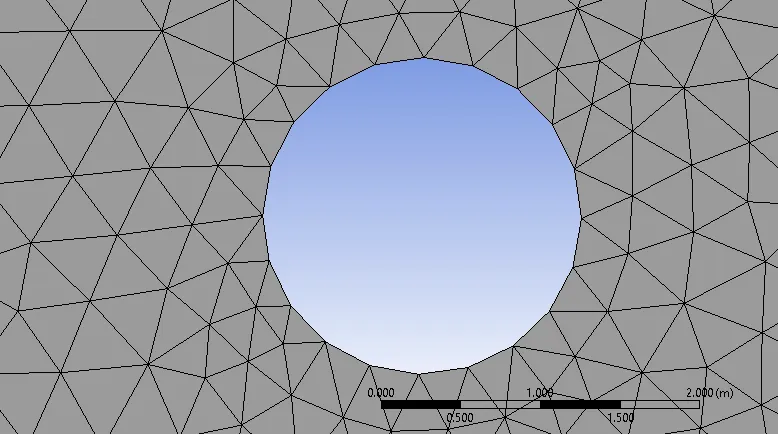
So, we have to insert the Sizing method to give a good shape to the cylindrical circle. I divide the cylinder into 36 parts.
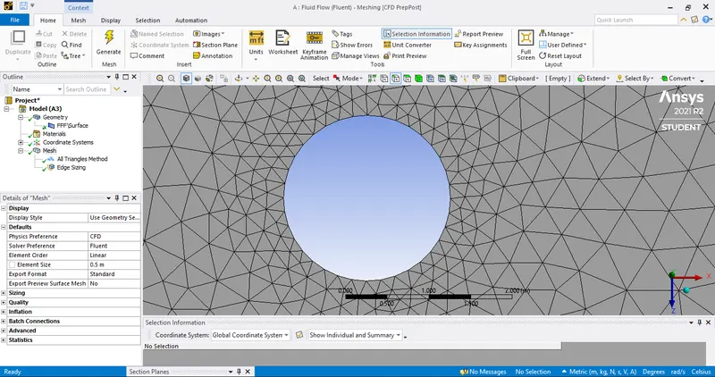
Now it is much better than previous one. But for better visualization of fluid flow near the wall we add more cells and to do that we add Inflation layer.
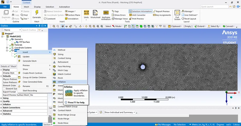
Here we add 12 inflation layer.
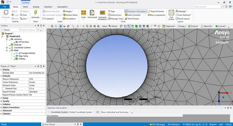
And again we increase the cells because we need more accurate results and that's why we need more fined mesh in our geometry. We give element size 0.2m.
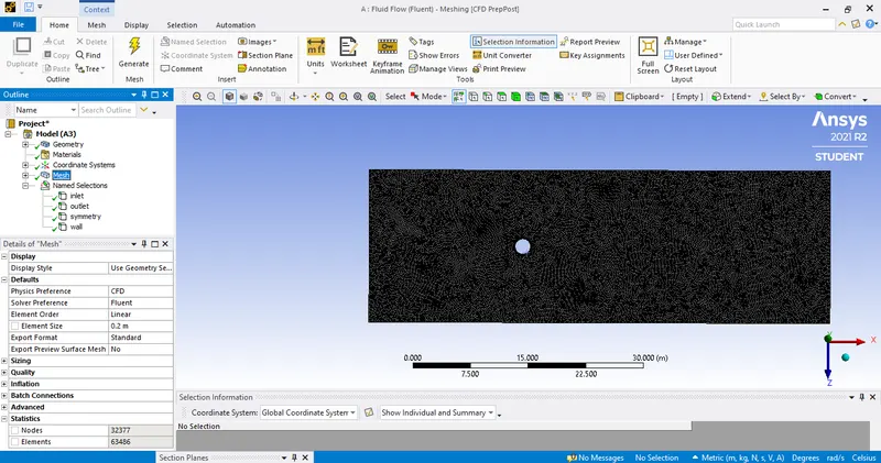
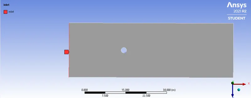
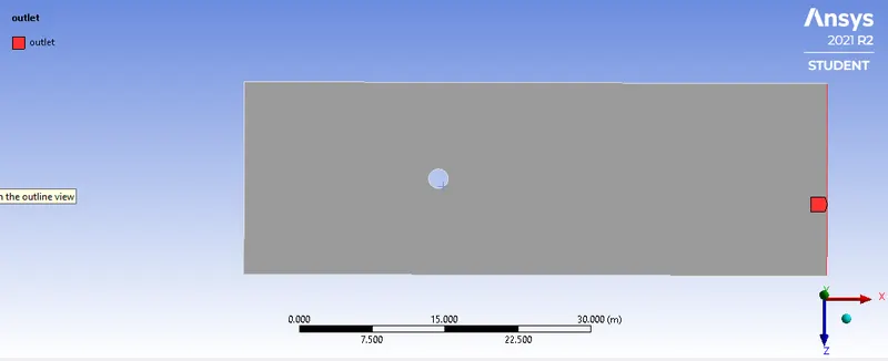
At last our meshing is complete and now we give the name of every edges of the geometry
1. Inlet
2. Outlet
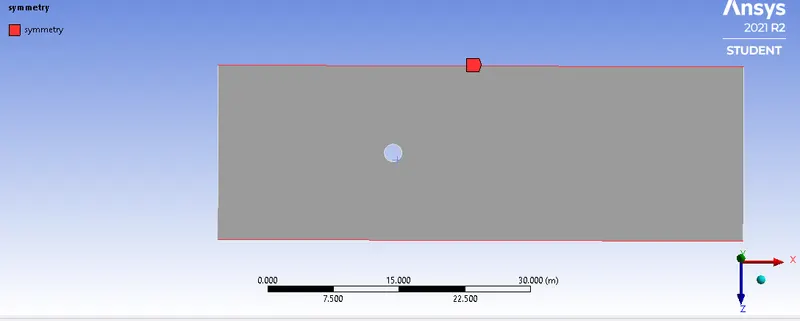
3. Symmetry
4. Wall
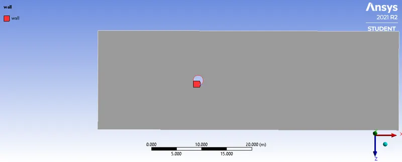
Thus we gave all the name of the geometry edge's.
Setting Up The Physics:- First we see the steady state simulation. The flow is laminar flow and we create the our own material which have density 1 and viscosity is 0.02. This user-material is our working fluid. And then we give the velocity 1 m/s. We create vortex average report, lift-coefficient and drag-coefficient report for our simulation. We initialized the initial conditions by Hybrid initialization method. Then we create velocity and pressure contours and also velocity annimation. And here we use SIMPLE method.
Material Properties
Material Properties
-------------------

   Material: user-material (fluid)

      Property                        Units      Method     Value(s)
      --------------------------------------------------------------
      Density                         kg/m^3     constant   1
      Cp (Specific Heat)              J/(kg K)   constant   1006.43
      Thermal Conductivity            W/(m K)    constant   0.0242
      Viscosity                       kg/(m s)   constant   0.02
      Molecular Weight                kg/kmol    constant   28.966
      Thermal Expansion Coefficient   K^-1       constant   0
      Speed of Sound                  m/s        none       #f

   Material: aluminum (solid)

      Property               Units      Method     Value(s)
      -----------------------------------------------------
      Density                kg/m^3     constant   2719
      Cp (Specific Heat)     J/(kg K)   constant   871
      Thermal Conductivity   W/(m K)    constant   202.4
Boundary Condition:-
Boundary Conditions
-------------------

   Zones

      name       id   type
      -------------------------------
      inlet      5    velocity-inlet
      outlet     6    pressure-outlet
      symmetry   7    symmetry
      wall       8    wall

   Setup Conditions

      inlet

         Condition                  Value
         --------------------------------
         Velocity Magnitude [m/s]   1

      outlet

         Condition   Value
         -----------------

      symmetry

         Condition   Value
         -----------------

      wall

         Condition                  Value
         ------------------------------------------
         Wall Motion                Stationary Wall
         Shear Boundary Condition   No Slip
Solver Settings
Solver Settings
---------------

   Equations

      Equation   Solved
      -----------------
      Flow       yes

   Numerics

      Numeric                         Enabled
      ---------------------------------------
      Absolute Velocity Formulation   yes

   Under-Relaxation Factors

      Variable      Relaxation Factor
      -------------------------------
      Pressure      0.3
      Density       1
      Body Forces   1
      Momentum      0.7

   Linear Solver

      Variable     Solver Type   Termination Criterion   Residual Reduction Tolerance
      -------------------------------------------------------------------------------
      Pressure     V-Cycle       0.1
      X-Momentum   Flexible      0.1                     0.7
      Y-Momentum   Flexible      0.1                     0.7

   Pressure-Velocity Coupling

      Parameter   Value
      ------------------
      Type        SIMPLE

   Discretization Scheme

      Variable   Scheme
      ------------------------------
      Pressure   Second Order
      Momentum   Second Order Upwind

   Solution Limits

      Quantity                    Limit
      ---------------------------------
      Minimum Absolute Pressure   1
      Maximum Absolute Pressure   5e+10
      Minimum Temperature         1
      Maximum Temperature         5000
Solution of Steady state simulation:-
Residual:- In the residual, we solve the equation of continuity, x-momentum and y-momentum
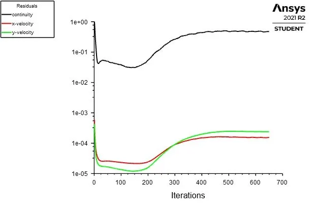
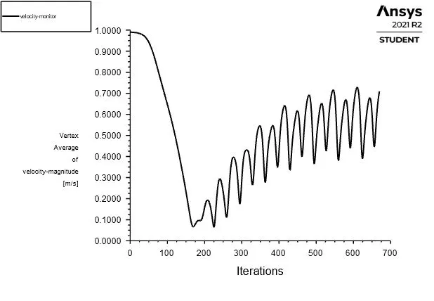
Vertex Average of Velocity Magnitude:- The vertex average of a specified field variable on a surface is computed by dividing the summation of the vertex values of the selected variable by the total number of vertices.
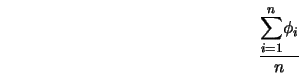
Here we calculate vertex average of velocity magnitude.
Lift Coefficient:-
Drag Coefficient:-
Velocity Contour:-
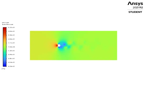
Pressure Contour:-
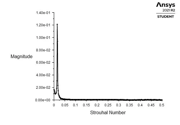
Strouhal Number:- Here in between 0 to 0.05 of Strouhal number, the magnitude is in the high pick. And where the magnitude is in high pick, this point is the value of Strouhal number at this time step.
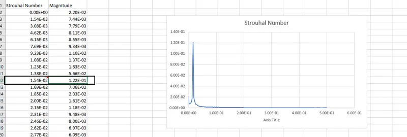
So the value of Strouhal number is 0.0154. And this is a excel sheet which show this
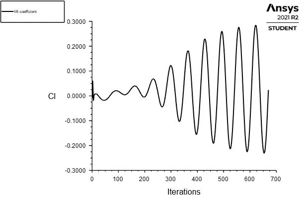
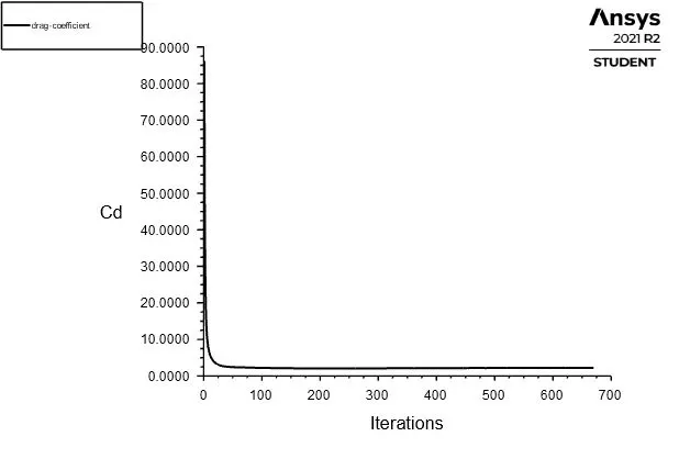
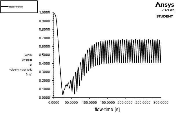
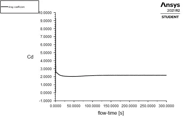
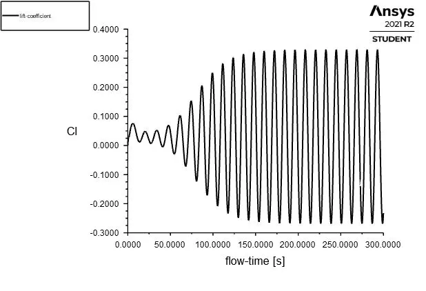
The values of Vertex Average of Velocity Magnitude, Lift Coefficient and Drag Coefficient:- Here, the Velocity monitor means the value of vertex average of velocity magnitude is 0.63885 m/s. The value of drag coefficient is 2.2138 and the value of lift coefficient is 0.20021 at 500 time step.

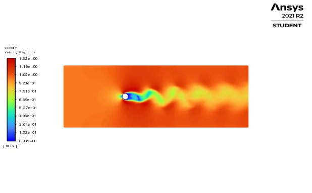
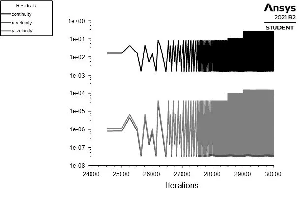
The Solutions of Transient Simulation of Re = 100:- All things are the same here, but the procedure we use is the Transient method. If we see the result of steady-state simulation, the vertex average of velocity magnitude shows a periodic motion that means the velocity of our working fluid is not constant with time. So, to track the velocity we have to consider the time because changing with time, the velocity is also changing. So, we have to do transient simulation to track the velocity properly.
Residual:- In the residual, we solve the equation of continuity, x-momentum and y-momentum and we see they are preodically goes up and down.
Vertex Average of Velocity Magnitude:-
Drag Coefficient:-
Lift Coefficient:-
Velocity Contour:-
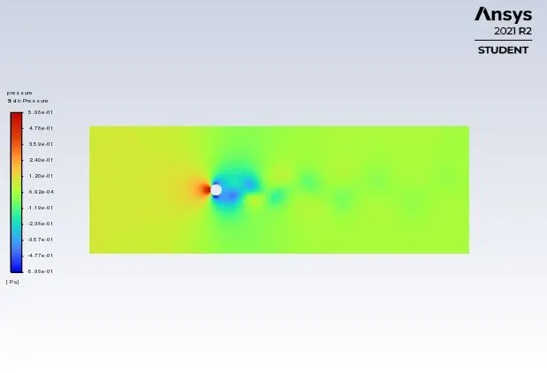
Pressure Contour:-
Strouhal Number:-Here in between 0 to 0.25 of Strouhal number, the magnitude is in the high pick. And where the magnitude is in high pick, this point is the value of Strouhal number at this time step.
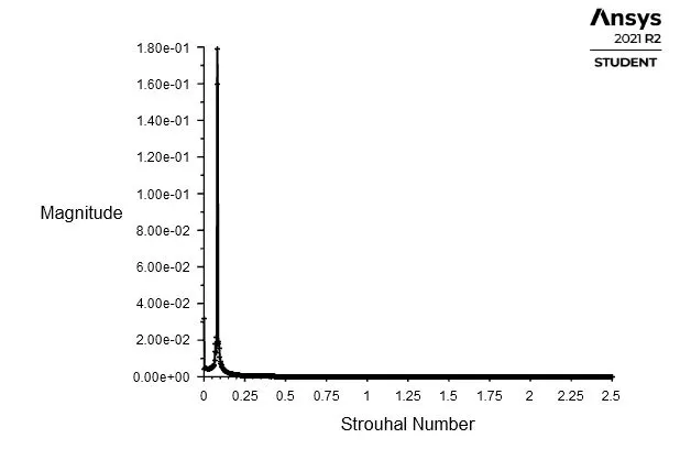
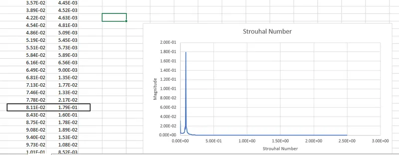
So the value of Strouhal number is 0.0811. And this is a excel sheet where we can see this
This is an annimation video for this simulation:-
Now we simulate the fluid flow over a cylinder in Reynolds numbers of 10,100,1000,10000 & 100000. In those simulation we mainly aware about the lift coefficient and drag coefficient.
For Re = 10:- In this simulation, the Geometry and Meshing procedures are same as previous. Because of Re = 10, the dynamic viscosity will be 0.2. And all other procedures are same as before.
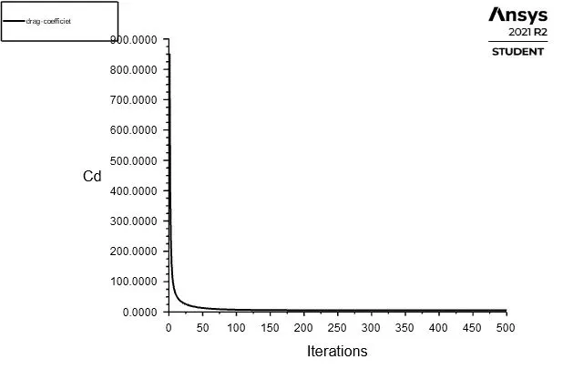
Drag Coefficient:-
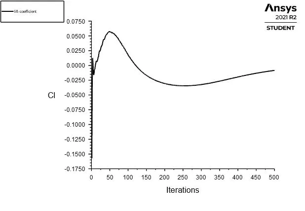
Lift Coefficient:-
Velocity Contour:-
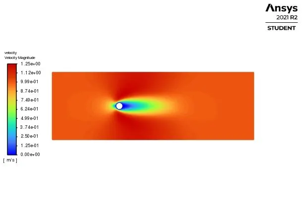
The calculated value of Vertex average of velocity magnitude, Lift coefficient and Drag coefficient:- Here, the Velocity monitor means the value of vertex average of velocity magnitude is 0.47146 m/s. The value of drag coefficient is 5.4868 and the value of lift coefficient is -0.0094084 at 500 time step.

The Simulation Of Fluid Flow Over A Cylinder For Re = 100(Steady Form):- We see the results of Re = 100 before. So, we now go for Re = 1000.
The Simulation Of Fluid Flow Over A Cylinder For Re = 1000(Steady Form):- Here also the geometry and meshing procedure same as previous simulation. But the dynamic viscosity is changed because of Renolds number is changed. The dynamic viscosity value is now 0.002 and all other value same as previous. Thr results are -
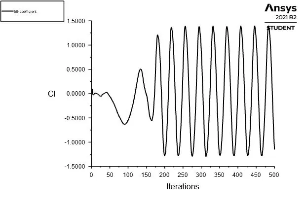
Lift Coefficient:-
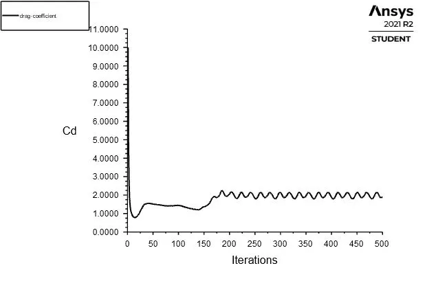
Drag Coefficient:-
Velocity Contour:-
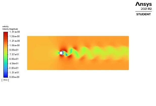
The calculated value of Vertex average of velocity magnitude, Lift coefficient and Drag coefficient:- Here, the Velocity monitor means the value of vertex average of velocity magnitude is 1.0394 m/s. The value of drag coefficient is 2.235 and the value of lift coefficient is -1.0138 at 500 time step.

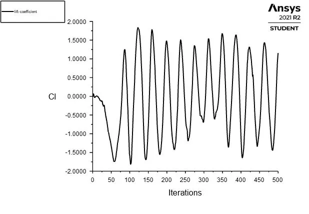
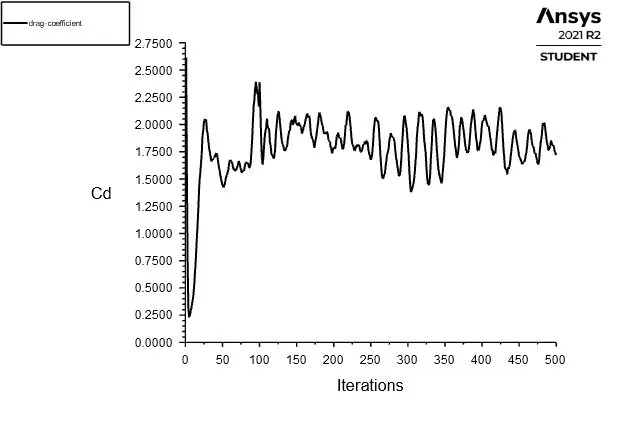
The Simulation Of Fluid Flow Over A Cylinder For Re = 10000(Steady Form):- Here also the geometry and meshing procedure same as previous simulation. But the dynamic viscosity is changed because of Renolds number is changed. The dynamic viscosity value is now 0.0002 and all other value same as previous. Thr results are -
Lift Coefficient:-
Drag Coefficient:-
Velocity Contour:-
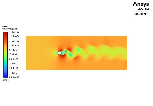
The calculated value of Vertex average of velocity magnitude, Lift coefficient and Drag coefficient:- Here, the Velocity monitor means the value of vertex average of velocity magnitude is 1.1163 m/s. The value of drag coefficient is 2.3414 and the value of lift coefficient is -0.5271.

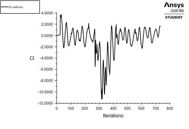
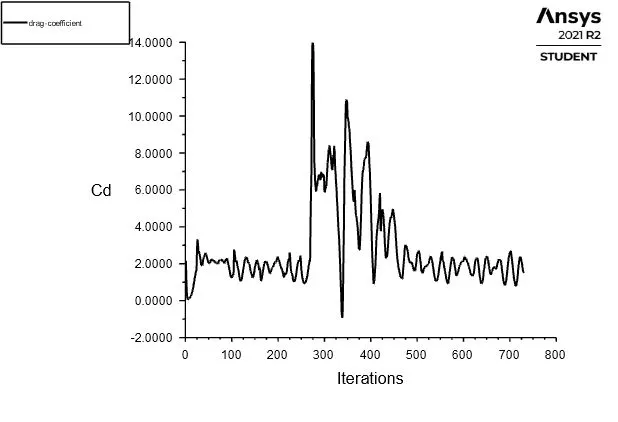
The Simulation Of Fluid Flow Over A Cylinder For Re = 100000(Steady Form):- Here also the geometry and meshing procedure same as previous simulation. But the dynamic viscosity is changed because of Renolds number is changed. The dynamic viscosity value is now 0.00002 and all other value same as previous. Thr results are -
Lift Coefficient:-
Drag Coefficient:-
Velocity Contour:-
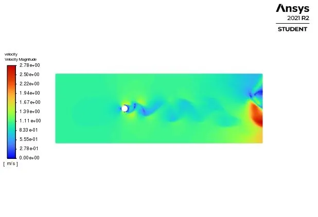
The calculated value of Vertex average of velocity magnitude, Lift coefficient and Drag coefficient:- Here, the Velocity monitor means the value of vertex average of velocity magnitude is 1.0817 m/s. The value of drag coefficient is 1.6058 and the value of lift coefficient is 0.63086 at 500 time step.

This is an annimation video for this simulation:-
Now, we discuss how Reynolds number affected the Drag Coefficient:- First, we see the results again in a summerize form for better understanding. We make a table of Reynold's number, Lift Coefficient, and Drag coefficient.
| Renolds Number | Lift Coefficient | Drag Coefficient |
| 10 | - 0.0094084 | 5.4868 |
| 100 | 0.20021 | 2.2138 |
| 1000 | -1.0138 | 2.235 |
| 10000 | -0.5271. | 2.3414 |
| 100000 | 0.63086 | 1.6058 |
And now we see the Drag coefficient plot of different Reynolds numbers.
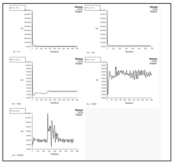
So, if we see the results then we can see that the drag coefficient continues to decrease with increasing Reynold's number in this range `10<= Re<=10^3`. Because the Reynold's number is inversely proportional to the Drag coefficient. We have some empirical relations for the drag coefficient
`C_D = 24/(Re)(1 + 0.0916Re)` for 0.1<Re<5
`C_D = 24/(Re)`
And these relations help us to prove our results and to prove our theory. We have also a graphical result of Drag Coefficient and Reynold's number
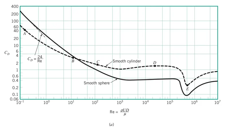
In the moderate range of `10^3<= Re <=10^5`, the drag coefficient remains relatively constant. This behavior is characteristic of bluff bodies. The flow in the boundary layer is laminar in this range, but the flow in the separated region past the cylinder is highly turbulent with a wide turbulent wake.
In our graph, there is a sudden drop in the drag coefficient in between the range of `10^5 <= Re <=10^6`(usually, at about `2*10^5`). This is due to the flow in the boundary layer becoming turbulent, which moves the separation point further on the rear of the body, reducing the size of the wake and thus the magnitude of the pressure drag.
Here we see the cylinder is smooth. In our case also the cylinder is smooth. That is because an increase in the surface roughness may decrease the drag coefficient. This is done by tripping the boundary layer into turbulence at a lower Reynolds number and thus delaying the flow separation, causing the fluid to close behind the body, narrowing the wake, and reducing the pressure drag considerably.
And now if we see the resultant plots of the Drag coefficient in dfferent Reynolds numbers, then we see with the increasing of Reynolds number the drag coefficient more unstable.
CONCLUSION:- So, we can now conclude our project.
- So, we calculate the Strouhal Number both in transient and steady-state of Re = 100. In a steady-state, the value of Strouhal Number is 0.0154, and in a transient state, the value of Strouhal Number is 0.0811.
- The Transient Simulation is more Preferable than the Steady-state for the Vortex Shedding phenomenon because it is time-dependent. With time, the flow velocity is changing.
- In Re = 10, we can’t see the vortex shedding that because when at about Re = 10 the flow separation starts occurring on the rear of the body with vortex shedding starting at about Re = 90. And the region of separation increases with increasing Reynolds number up to about Re = `10^3`.
- When the Reynold's number is small, the flow behaves like a potential flow. But with the increase of Reynold's number, the drag coefficient is decreasing and it’s going to be more unstable.