Week 2 - Flow over a Cylinder.

Aim:-- Simulate the flow over a cylinder and explain the phenomenon of Von-Karman vortex street.

Von-Karman Vortex Street

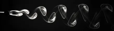
--> When a fluid (like air or water) flows externally over a structural body a wake region is formed behind the body. The wake region is the Viscous stress dominated region where the velocity is lower than the free stream velocity and the flow outside this region is accelerated to bring the average cross-sectional velocity back to free-stream velocity. The wake region is formed as a result of flow separation across the body which is caused by an Adverse pressure-gradient (which is mainly due to the geometry[reducing cross-section] of the body).

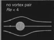
--> At different values of Reynolds Number a wide range of flow patterns are observed in the Wake region. At a very low Reynolds Number (Re<4) the flow divides and reunites smoothly with symmetry w.r.t the body. Flow is fully laminar and the wake region is not formed. At Re=>4 for circular cylinders, the flow separates at downstream and two steady standing eddies are formed in the wake region. These eddies are stable and remain attached to the body. This flow is invariant in time(steady flow).

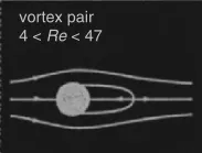
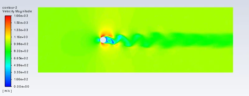
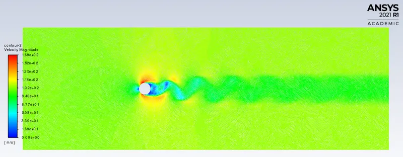
--> For circular cylinders At Re=>40 (Re(cr)=47) eddies in the wake become unstable and oscillations start to grow with increasing Reynolds number. Oscillation starts to grow and vortices are shed off from the eddies alternatively creating a high-pressure low-pressure region in the wake. This process is known as Vortex Shedding. In fluid dynamics, a Kármán vortex street is a repeating pattern of swirling vortices caused by vortex shedding in the trail of wake region.

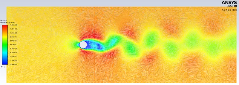
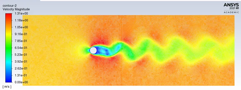
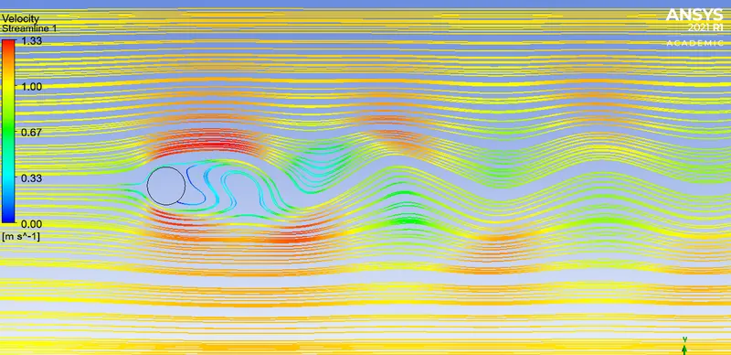
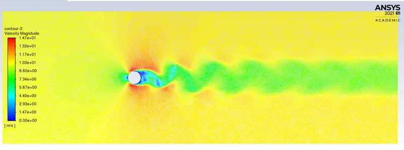
--> Vortex shedding flow is an unsteady flow (time-dependent) as the flow properties change with time(periodically). We need to make a Transient analysis for this problem. This flow gives rise to asymmetric top-to-bottom pressure-distribution causing fluctuations in the lift force. We can see that the vortices detach periodically forming discrete spaced vortices downstream.

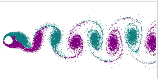
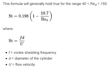
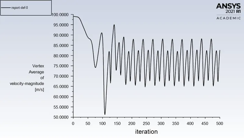
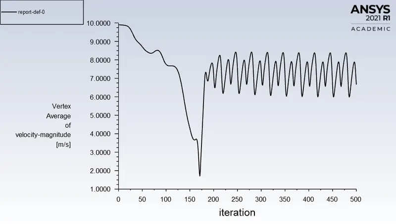
--> If we placed a velocity-measuring instrument in the wake, it would show a regular oscillation with one cycle corresponding to the distance between two vertices of the same sign. The frequency of this oscillation, when nondimensionalized by the diameter and the free-stream speed, is called the Strouhal (St) number. The Strouhal number varies slightly with Re but is roughly 0.2 over a wide range in Re.

The Strouhal number represents the ratio of inertial forces due to the local acceleration of the flow to the inertial forces due to the convective acceleration.

Pre-Processing step:

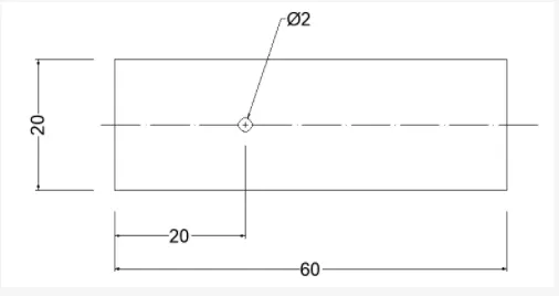
The model was designed in Ansys SpaceClaim, the sketch with dimensions are shown below.

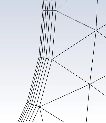
A mesh element of 0.2 m was used to generate the mesh in Ansys meshing. Further refinement of the mesh was done by using the triangulation method and sizing parameters of the hole were redefined for better geometry and meshing. Inflation layers were also added near the wall to capture the effect of the wall.

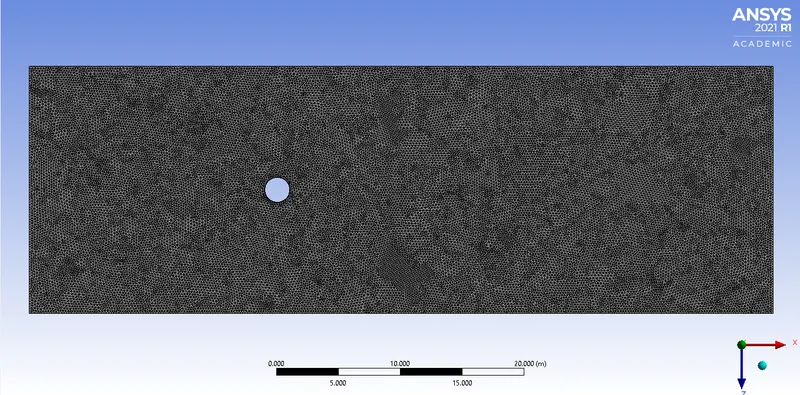
Mesh near wall Inflation Layer

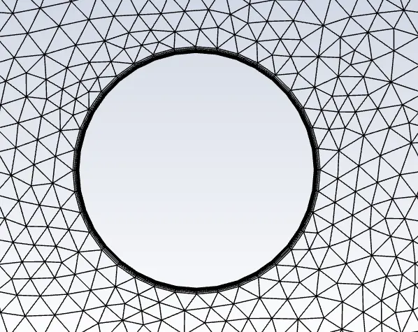
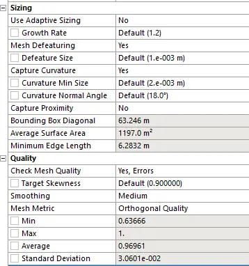
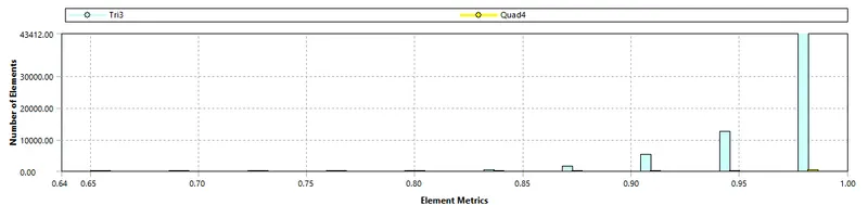
Mesh Metric plot for Mesh quality. (Orthogonal quality)

Material Used: Air

Properties: density=1kg/m^3 viscosity=0.02Kg/m-s

Outlet Pressure = 0 Pa (Gauge)

wall --- no slip

velocity (m/s) = 0.1 , 1 , 10 , 100 , 1000

PART-I

1. Simulate the flow with the steady and unsteady case and calculate the Strouhal Number for Re= 100.

TRANSIENT CASE vs STEADY-STATE CASE

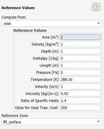
-->With Inlet velocity 1 m/s and Reynolds number 100, we carry out the simulations for both steady and transient case. The reference data is as shown--->

RESIDUALS:

Transient

Steady

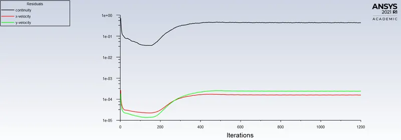
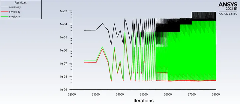
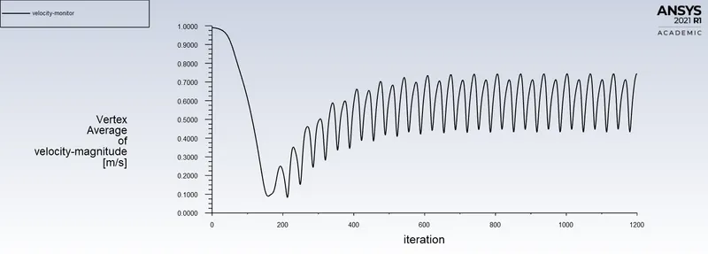
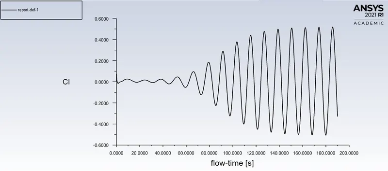
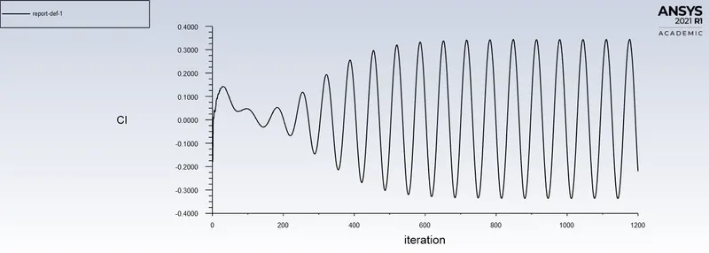
For Transient state, we took time step size 0.1 seconds and no. of time steps 1900. For steady-state no. of Iterations were 1200. We can see that in steady-state convergence takes place within 500 iterations. Steady-state solutions are only used to check the end result and any result in between is not accurate in time. For the convergence of the Transient case, the repetition of residuals can be considered as a convergence after some time steps.

Velocity:

Transient

velocity at the monitor point.

Velocity Contour(Transient)

Steady

velocity at the monitor point.

Velocity Contour(Steady)

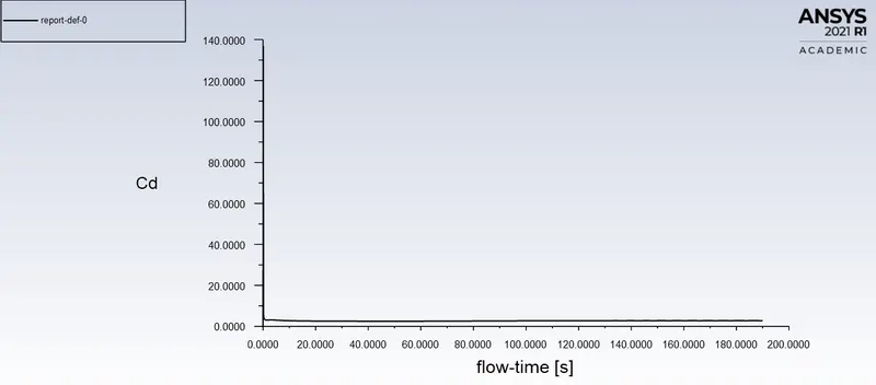
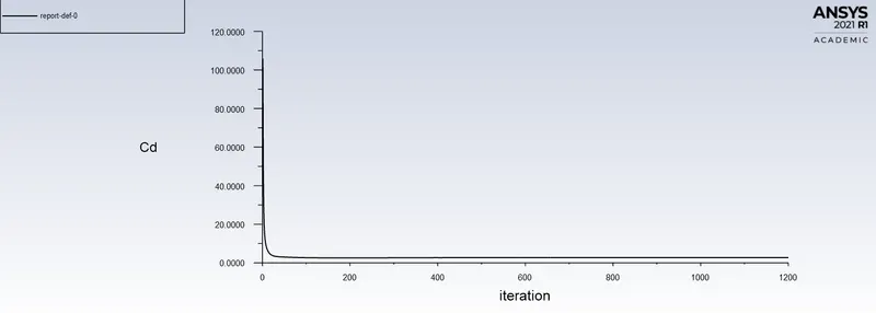
DRAG-COEFFICIENT

Transient

Steady

LIFT-COEFFICIENT

Transient

Steady

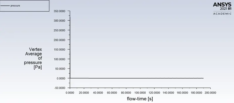
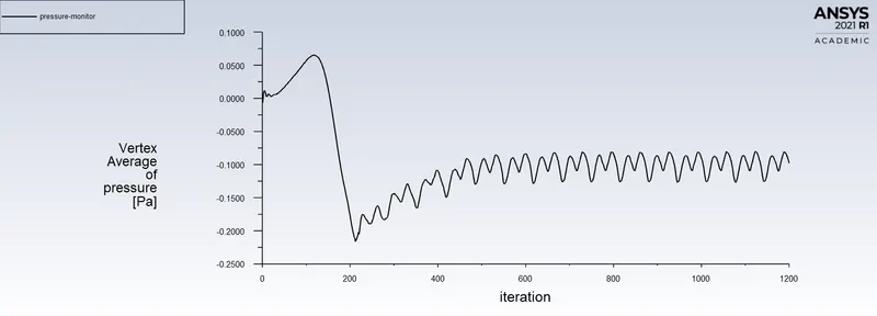
Pressure:

The pressure at the monitor point.

Transient case

Steady-state case

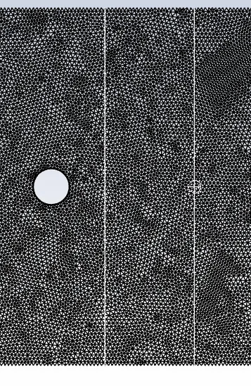
A monitor-point was added 8 meters downstream, a vertical line passing through the monitor point along the cross-section was added and another line was added near the cylinder wall at 3 meters. These are shown below:--

Near-wall line; Monitor line; Monitor point;

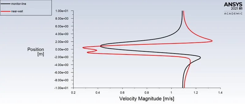
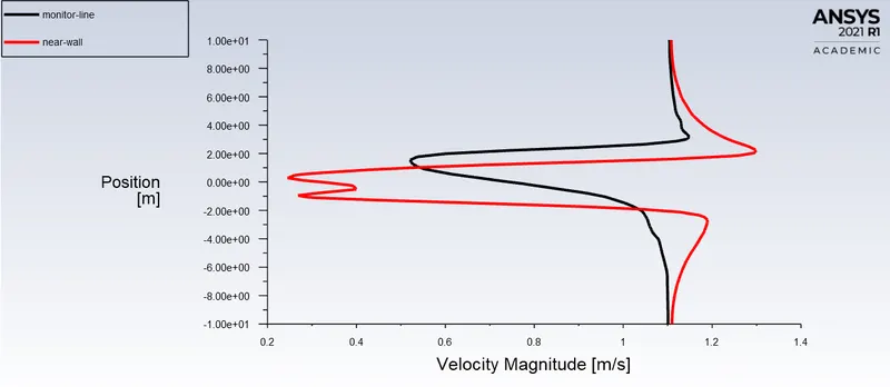
Velocity Profile Graph at the vertical lines placed at 3m(red) and 8m(black)

Transient Steady

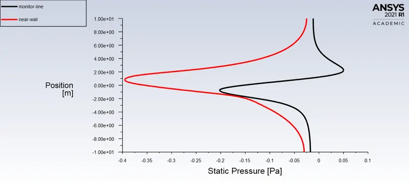
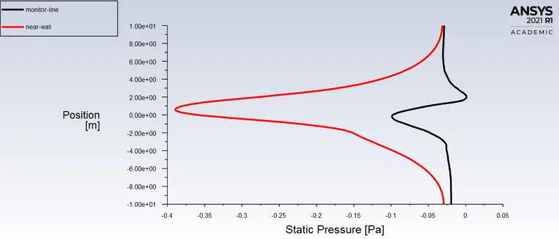
Pressure Profile Graph at the vertical lines placed at 3m(red) and 8m(black)

Transient Steady

Strouhal Number:

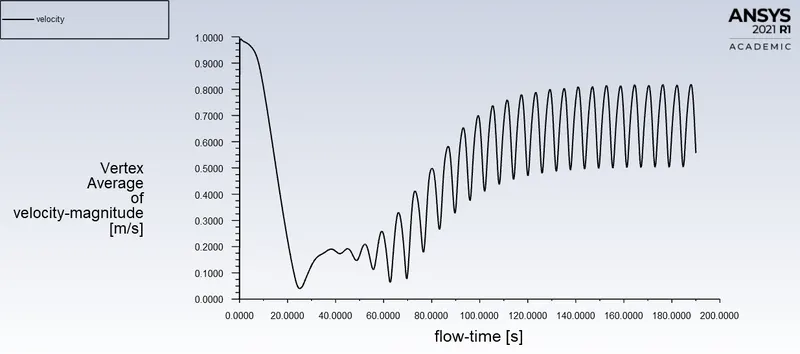
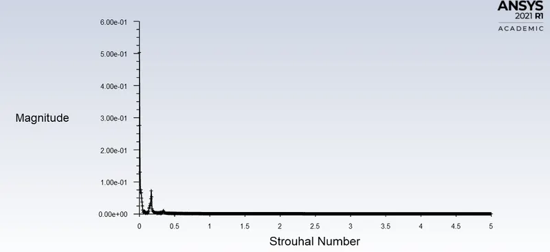
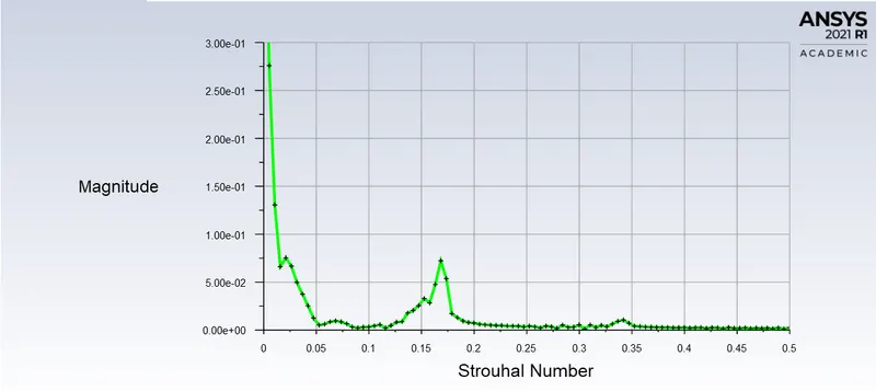
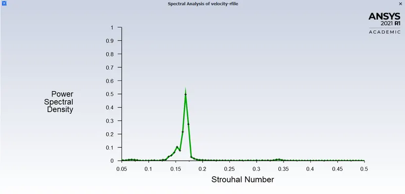
As we place the probe monitor point and obtain the velocity at monitor point downstream w.r.t time step we can calculate the strouhal number. This can't be done in steady-state as intermediatory results are not accurate with time. We generate the FFT (Fast Fourier transform) of the report velocity plot which contains the oscillations recorded downstream.

st (strouhal no.) = 0.17

Pressure Distribution Across the cylinder-->

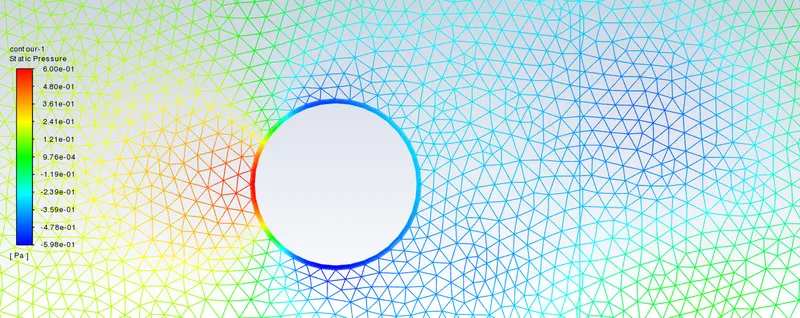
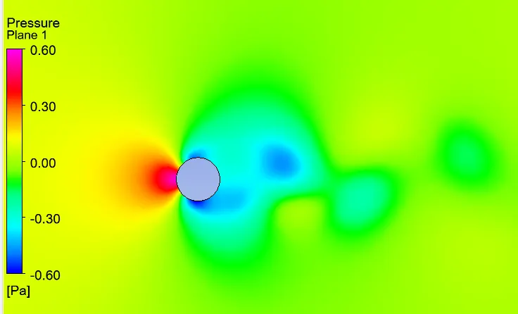
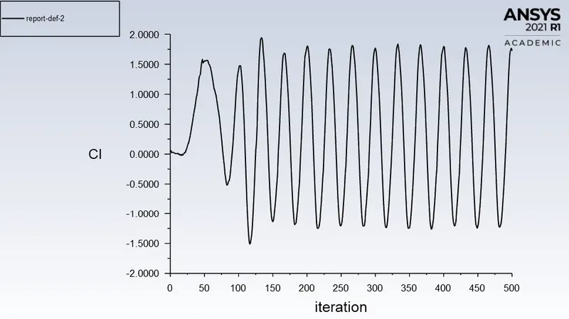
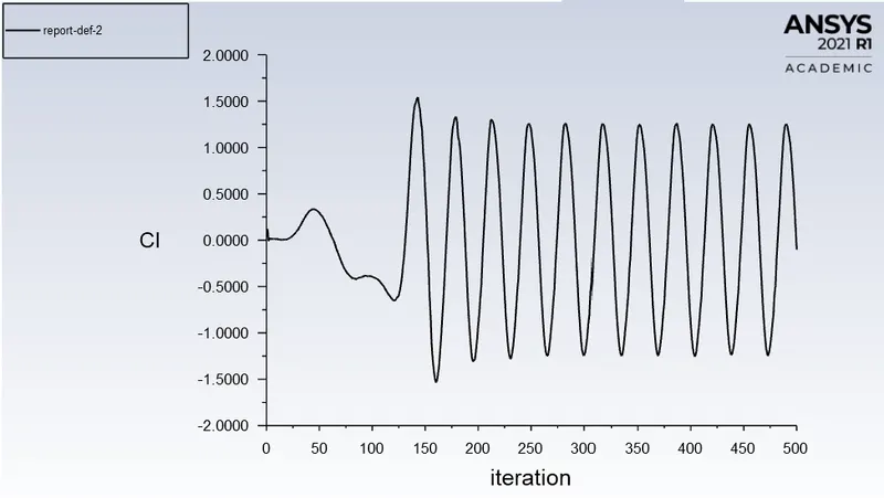
--> As we can see the pressure distribution across the cylinder, in the upstream part of the cylinder we have a favourable pressure-gradient (negative pressure-gradient) and in the downstream part of the cylinder we have an adverse pressure-gradient (positive pressure-gradient) i.e. pressure increases in the downstream part of the cylinder causing the flow to separate. Moreover, we can see pressure imbalance created at the top and bottom of the cylinder generating lift force and also in upstream and downstream part generating drag force(pressure-drag). Lift force is oscillating in nature.

Velocity-Streamline plot

PART-II

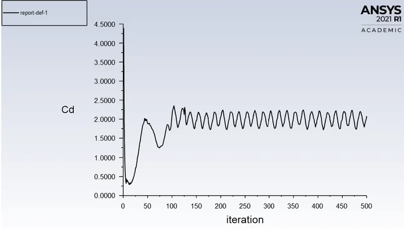
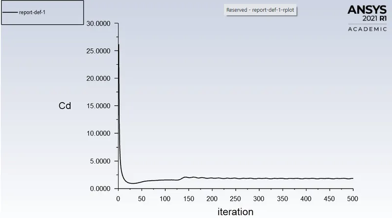
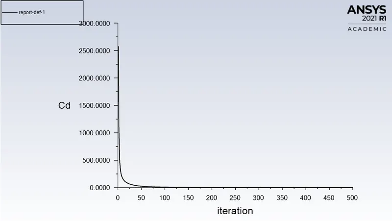
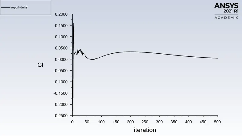
1. Calculate the coefficient of drag and lift over a cylinder by setting the Reynolds number to 10,100,1000,10000 & 100000. (Run with steady solver)
2. Discuss the effect of Reynolds number on the coefficient of drag. [ Results should be validated with any standard literature and error should be within 5 %]

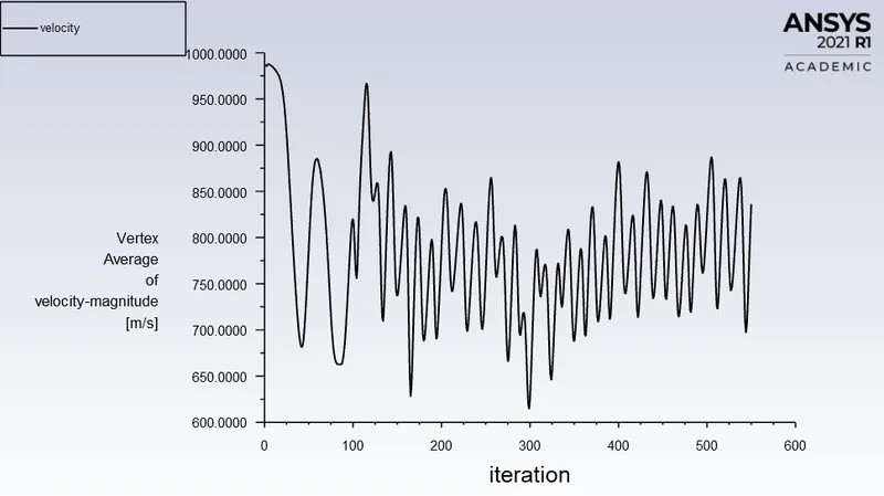
1. For Re=100000

monitor-velocity plot

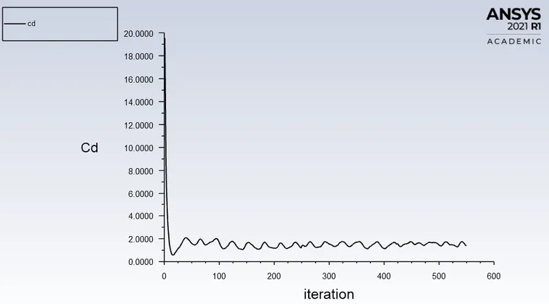
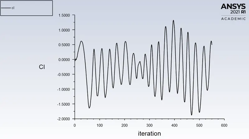
Coeff. of Drag and Lift plots

Velocity contour

1. For Re=10000

monitor-velocity plot

Coeff. of Drag and Lift plots

Velocity contour

1. For Re=1000

monitor-velocity plot

Coeff. of Drag and Lift plots

Velocity contour

1. For Re=100

monitor-velocity plot

Coeff. of Drag and Lift plots

Velocity contour

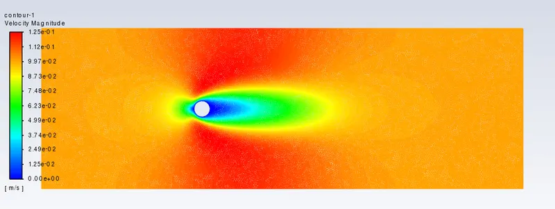
1. For Re=10

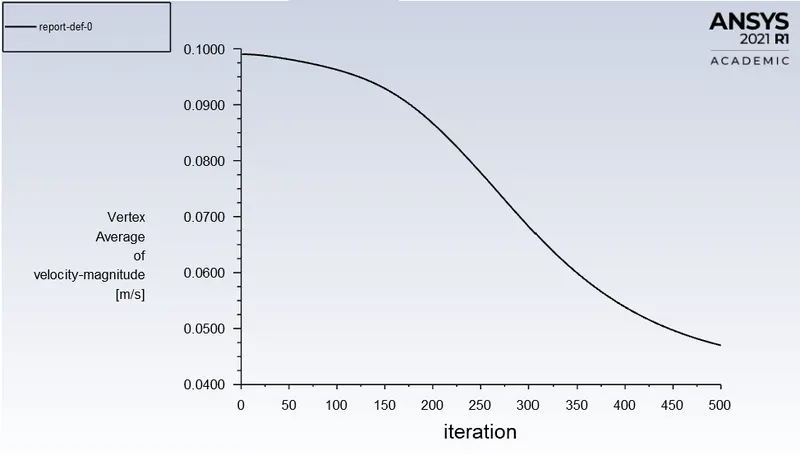
monitor-velocity plot

Coeff. of Drag and Lift plots

Velocity contour

Reynolds Number	Coefficient of Drag Cd	Coefficient of Lift Cl
100000	1.44	0.49
10000	1.72	1.6
1000	1.96	-0.023
100	2.7	-0.22
10	6.7	0.0044

--> From the above Table it can be concluded that if we increase the Reynolds number the coefficient of drag reduces.

-->For the higher value of Reynolds number, we also see oscillations in drag coefficient.