Week 2 - Flow over a Cylinder.
Aim
Simulate the flow over a cylinder and Study the vortex shedding phenomenon.
Objectives
- Explain the phenomenon of Karman Vortex Street.
- Simulate the flow with the steady and unsteady case and calculate the Strouhal Number for Re= 100.
- Calculate the coefficient of drag and lift over a cylinder by setting the Reynolds number to 10, 100, 1000, 10000 & 100000 using a steady-state solver
- Discuss the effect of Reynolds number on the coefficient of drag.
- Plot the lift and drag coefficients, convergence and show vortex shedding behind the cylinder in each case
Methodology
In order to perform this 2D laminar flow over a cylinder, Ansys Fluent from Ansys Workbench has been used. The solver solves the governing equations, which include momentum, energy equations, etc. with the help of some additional equations as per the type of simulation that we are going to perform.
According to the problem definition, we will study the flow of the cylinder at different Reynolds numbers. As the problem is solved we will understand the phenomenon of vortex shedding as per Karman Vortex Street.
Karman Vortex Street: When a blunt body is placed in a free stream fluid such as air or water, depending upon the size of the object and the velocity of the free stream, a vortex flow will take place just behind the object. This will create a low-pressure area behind the object causing the object to move towards it. This is called as Von-Karman Vortex Street. As per Von Karman, when the Reynolds number is above 90 in Laminar flows, the flow will start to generate vortex shedding. We will study this using an example in this project.
Strouhal Number: Strouhal Number is a non-dimensional parameter that describes the oscillation flow mechanism. The Strouhal number is calculated from the frequency of oscillation, characteristic length of the body, and free stream velocity. It is obtained by converting a sequence of data in the time domain to its frequency domain.
Strouhal Number `t=(fl)/u ;`
Where,
`f=` Frequency of vortex shedding
`l=`Characteristic length
`u=`Free stream velocity
Preprocessing
Step 1: Geometry creation
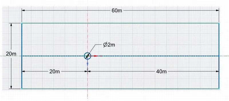
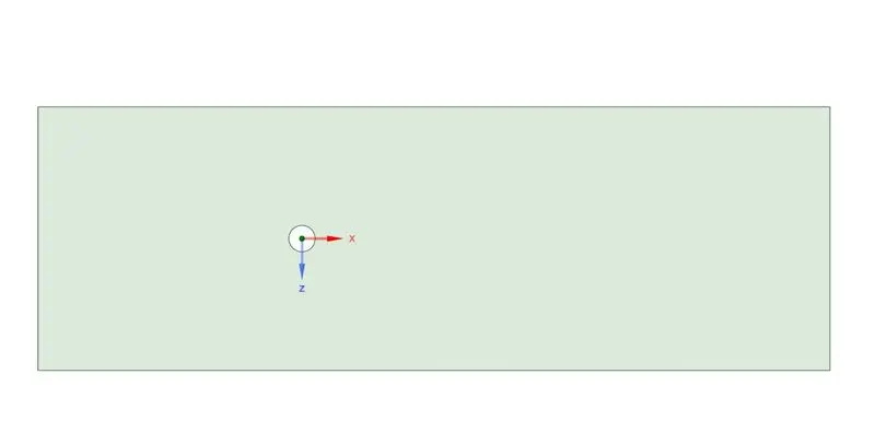
The following geometry has been created by using Spaceclaim in ansys fluent module.
The diameter of the cylinder is taken a 2m and a fluid domain has been created around the cylinder as per the diagram shown below.
Step 2: Naming and meshing of the fluid domain
After creating the geometry file the next step is to divide the domain into small elements. Before that, we will assign names for different faces to apply boundary conditions easily. After that, the mesh has been generated by clicking on generate mesh.
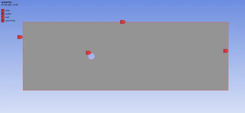
By default, ansys will create quadrilateral elements for 2D geometry. Since it won’t capture all the area around the cylinder we will make triangular elements and will refine the meshed near the cylinder wall.
To create the triangular mesh, right-click mesh, go to insert, click on methods, select geometry, then change methods to triangles.
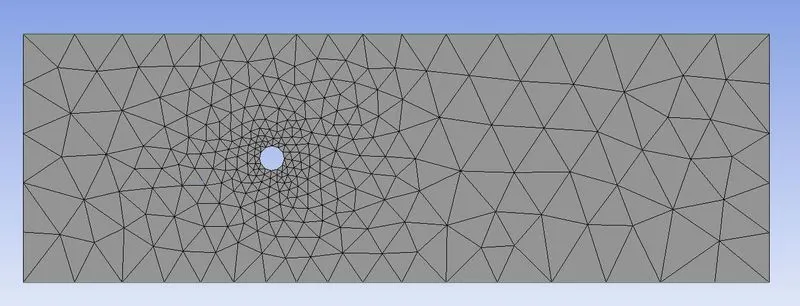
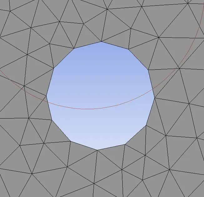
We can see a coarse mesh has been formed. If we look near the circular edge we can see that the edge looks like a polygon shape rather than a circle. To refine this circular edge, right-click mesh, click on insert, click on sizing. Under geometry, select the circular edge. Under type, change it to the number of divisions. Put the number of divisions as 36, because this will create a good circular edge. Now update the mesh to see the new mesh.
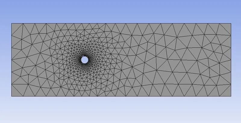
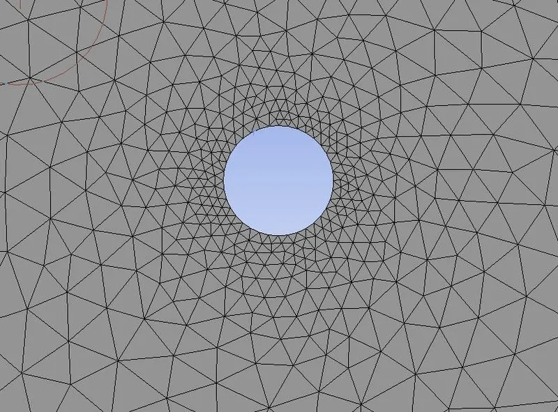
Since the flow around the cylinder is very important, we need to take care of the region around the cylinder. For this purpose, inflation layers are created around the cylinder. This will create offset layers around the cylinder.
Right-click mesh, click on insert, click on inflation. Now select our body for geometry and select circular edge as a boundary. Under inflation, options select first layer thickness. Give 0.005m as the first layer thickness and select maximum layers as 6. Now update the mesh.
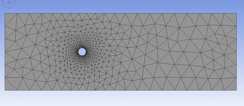
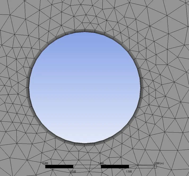
As the mesh is updated we can see that 6 layers have been formed around the cylinder.
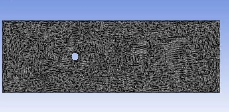
Change the element size to 0.25mm under mesh properties to obtain a fine mesh
Step 3: setting up the problem.
Here we set up the problem by applying relevant
- Initial conditions
- Boundary conditions
- Material properties
- Turbulence Models
Material Properties.
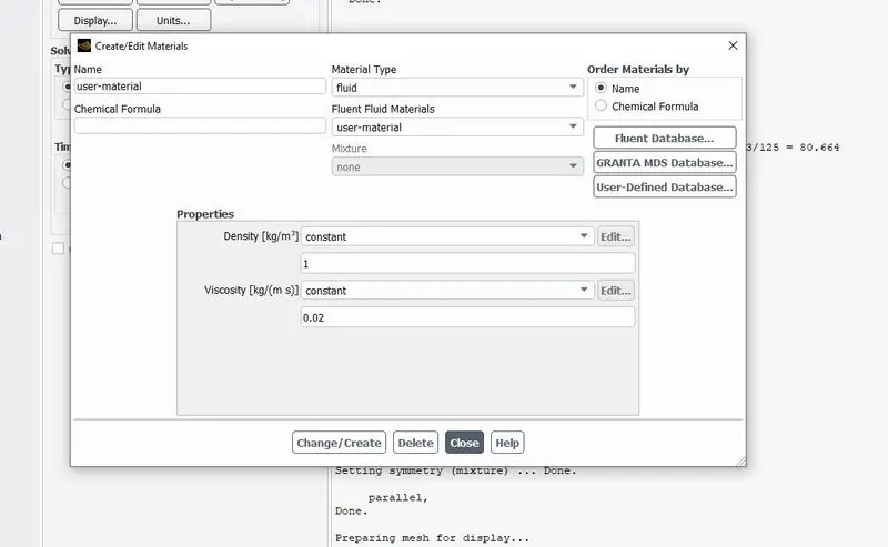
A user-defined material is created to solve all the problems. The same material is used for all the cases.
Density =`1 kg//s`
Kinematic viscosity =`0.02 kg//ms`
All other properties are like Air.
Turbulence Model:
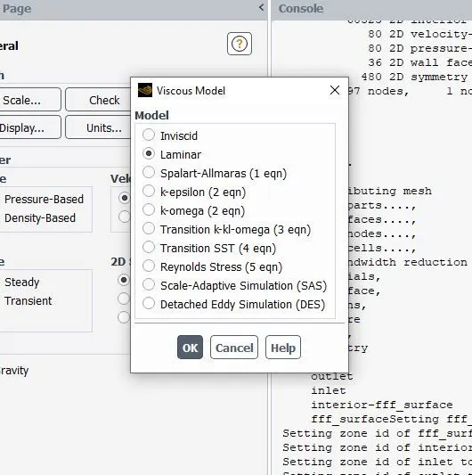
Since the flow is Laminar we are taking laminar as the viscous model.
Initial and boundary conditions
We will set up initial and boundary condition’s as we solve each case.
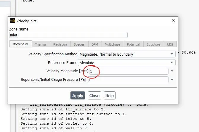
Inlet - Velocity boundary condition: Here the velocity magnitude will be changed as per the Reynolds number required. From 0.1 to 1000 m/s.
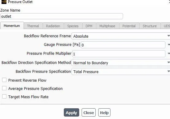
Outlet - Pressure outlet: Gauge pressure = 0
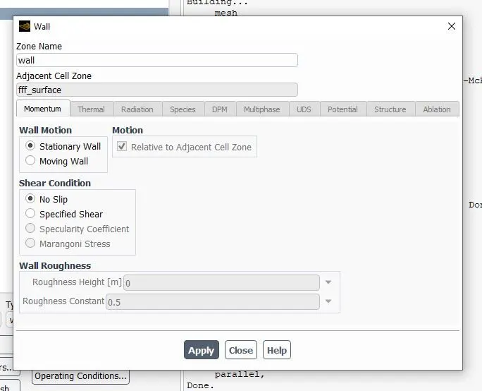
Wall – No slip
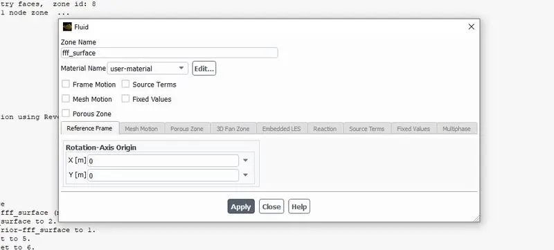
Ensure that in the cell zone, the fluid used is user material.
Reference Values
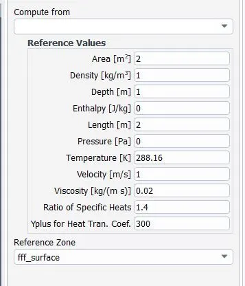
As we have modified our material properties we need to modify the reference values also.
Click on reference values under physics. Click on the inlet in the compute from the drop-down. Ensure that the area, density, velocity, and viscosity are as per our values. The area is nothing but the projected area. In our case, it is 2.
Setting up Result extraction
Before running the simulation let’s set up some plots and curves for extracting results as the simulation proceed.
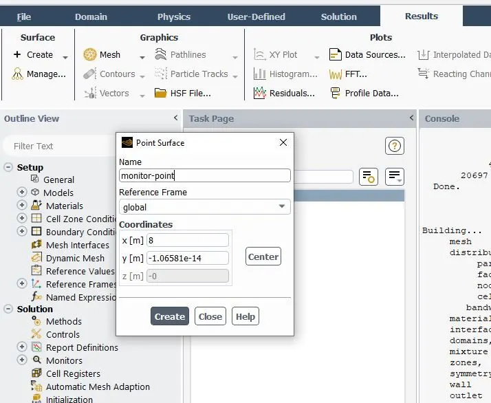
As we are interested in the physics after the fluid has passed the cylinder, we will create a monitor point 8m behind the cylinder. Then, we will define vertex averaged velocity at that monitor point. To study the lift and drag coefficients on the cylinder wall we will define lift and drag coefficient plots also.
Creating Monitor point:
Go to results, click on create, then point. Change the name as monitor-point. Put x distance = 8
After creating the monitor point Different plots have been defined using the definition tool under solution.
In order to see the Velocity and pressure contours are evolving while solving, we are creating contours before running the simulation.
For that, first, we need to initialize the solution so that the solver gets the initial values of pressure and velocity. Later contours are defined from the results menu. The contour option will not be visible if the solution is not initialized.
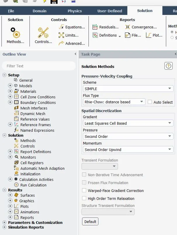
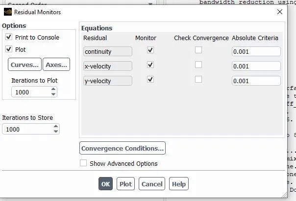
After all the above steps let’s change the solution method to a simple scheme. Uncheck all the convergence in the residual menu since we want to see the solution till the completion of all iterations. Then input the number of iteration=1000 to start the simulation.
PART 1: Simulate the flow with the steady and unsteady case and calculate the Strouhal Number for Re= 100.
- Steady case
Diameter D = `2m`
Density `rho = 1kg//m^3`
Viscosity `mu=0.02kg//ms`
Reynolds number `Re = 100`
Velocity `u=(Re*mu)/(rhoD) = 1m//s`
Number of iterations = 1000
- Solutions
- Residual plot
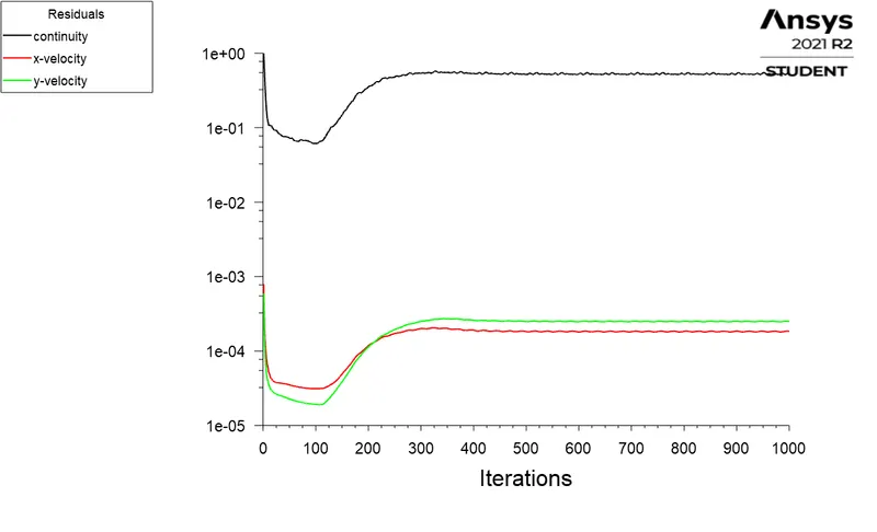
From the residual plot we can see that continuity and momentum equations are converged after 500 iterations. It means that the flow has converged.
Velocity at the monitor point
The monitor point is 8m away from the cylinder as mentioned.
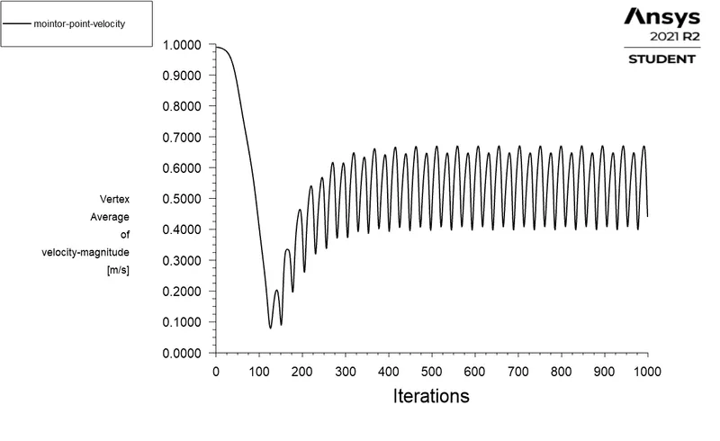
From the above plot, we can say that after some iterations the velocity at the monitor point has been converged. It is also noted that the velocity is oscillating. This can be further understood in contour plots.
3. Coefficient of drag
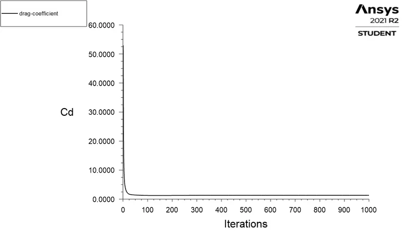
The coefficient of drag = 1.3429
4. Coefficient of lift
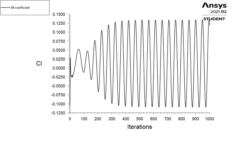
The coefficient of lift = 0.1191
5. Velocity Contour
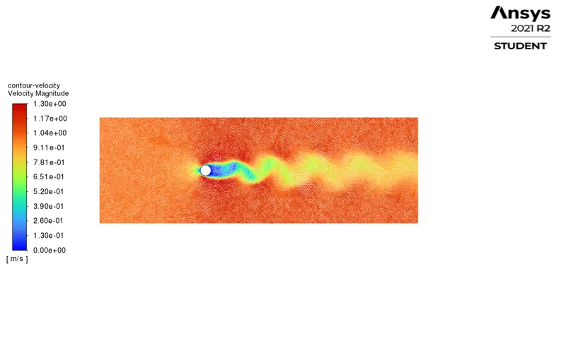
The Velocity contour shows that there is vortex shedding behind the cylinder. It is also noted that the vortex shedding happened when the Reynolds number is 100, which justifies the Von-Karman vortex theory.
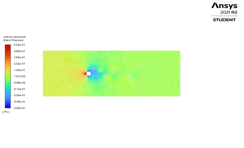
6. Pressure Contour
B. Unsteady case
Diameter D = `2m`
Density `rho = 1kg//m^3`
Viscosity `mu=0.02kg//ms`
Reynolds number `Re = 100`
Velocity `u=(Re*mu)/(rhoD) = 1m//s`
Time step size = 0.25s
Number of Time steps = 1000
- Solutions
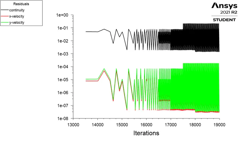
Residual plot
Velocity at the monitor point
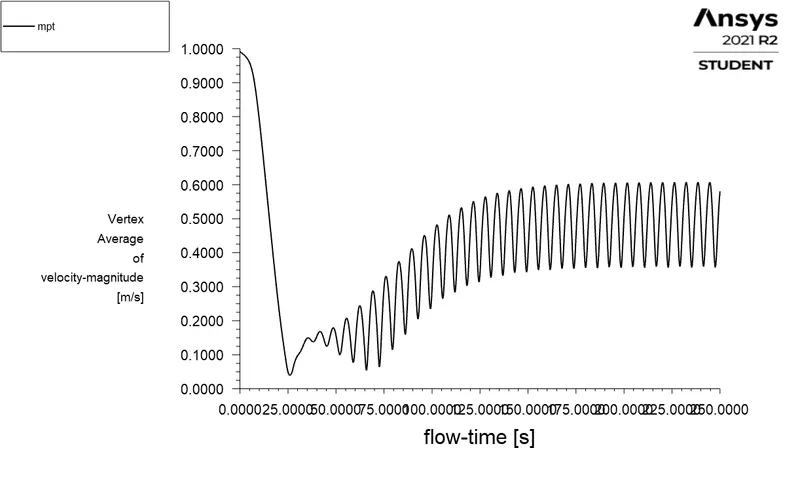
We can observe that the velocity at the monitor point is oscillating within a upper and lower limit after 150 seconds. Which means that the solution has converged
Coefficient of drag
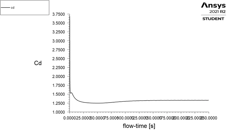
The coefficient of drag = 1.3304168
Coefficient of lift
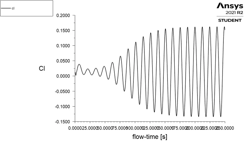
The coefficient of lift = 0.14331805
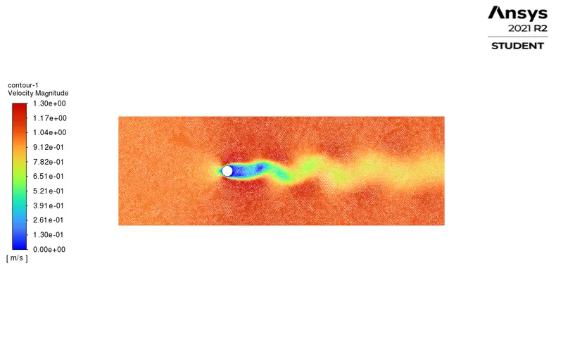
Velocity contour
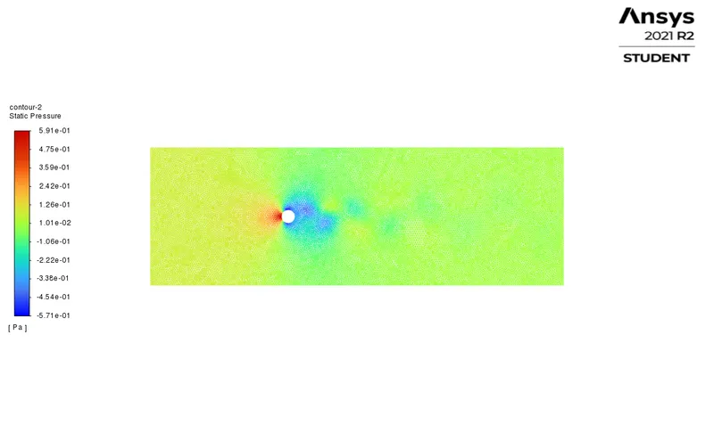
Pressure Contour
Strouhal Number
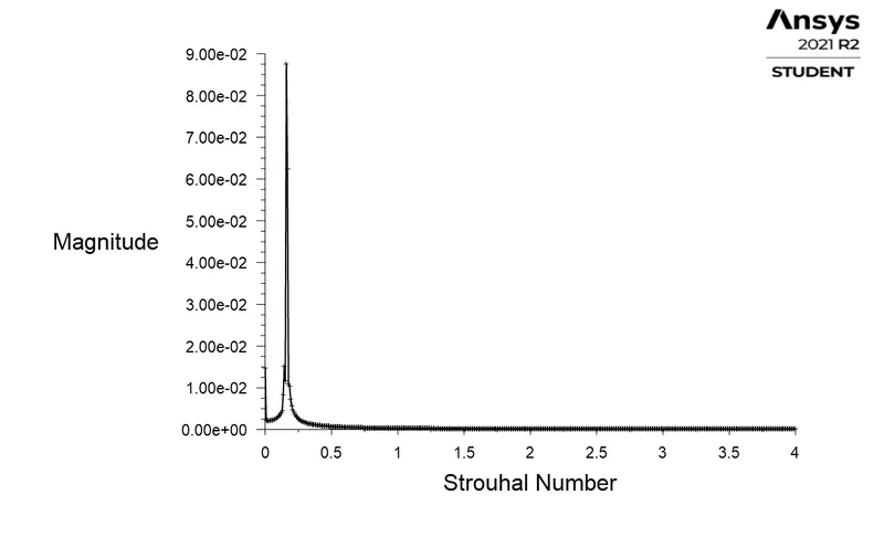
Strouhal Number = 0.15984017
PART 2 Calculate the coefficient of drag and lift over a cylinder by setting the Reynolds number to 10,100,1000,10000 & 100000
- Re = 10
Diameter D = `2m`
Density `rho = 1kg//m^3`
Viscosity `mu=0.02kg//ms`
Reynolds number `Re = 10`
Velocity `u=(Re*mu)/(rhoD) = 0.1m//s`
Number of iterations = 1000
- Solutions
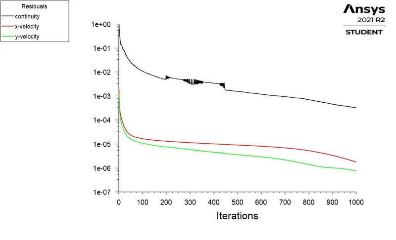
1. Residual plot
2. Velocity at the monitor point
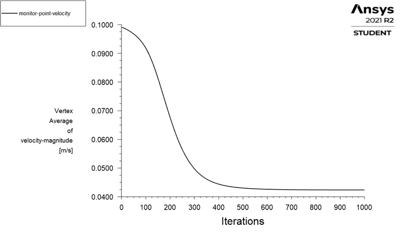
From the above plot, we can say that after some iterations the velocity at the monitor point has been converged.
3. Coefficient of drag
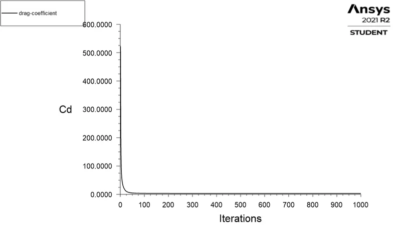
The coefficient of drag = 3.3242022
4. Coefficient of lift
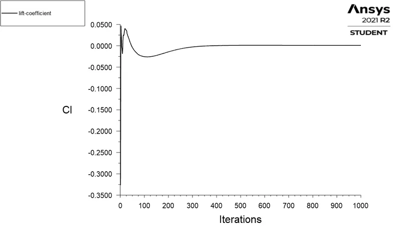
The coefficient of lift = 0.00092959535
5. Velocity contour
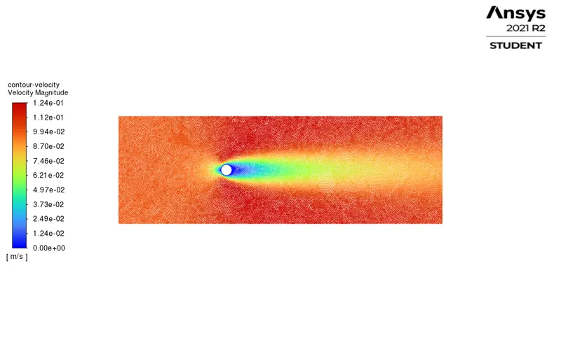
The Velocity contour shows that there is no vortex shedding behind the cylinder.
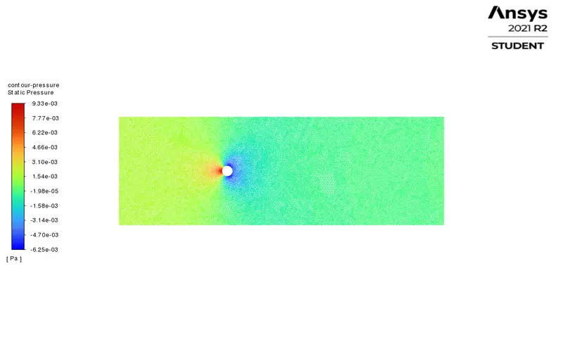
6. Pressure contour
2. Re = 1000
Diameter D = `2m`
Density `rho = 1kg//m^3`
Viscosity `mu=0.02kg//ms`
Reynolds number `Re = 1000`
Velocity `u=(Re*mu)/(rhoD) = 10m//s`
Number of iterations = 1000
- Solutions
1. Residual plot
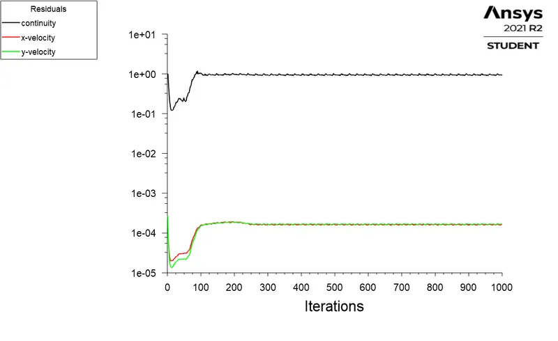
2. Velocity at the monitor point
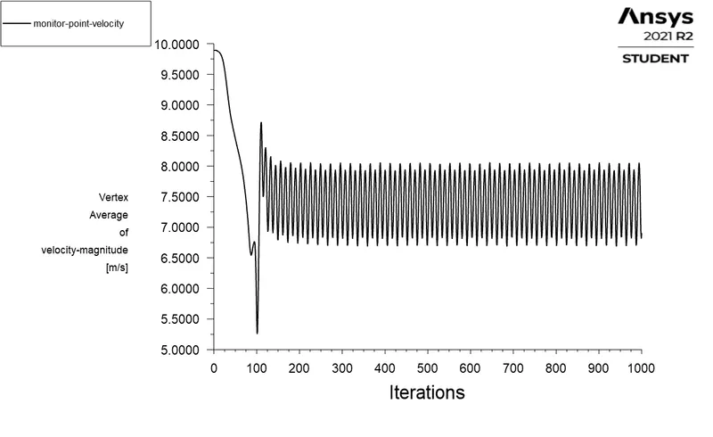
From the above plot, we can say that after some iterations the velocity at the monitor point has been converged. It is also noted that the velocity is oscillating. This can be further understood in contour plots.
3. Coefficient of drag
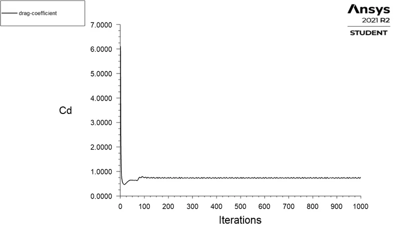
The coefficient of drag = 0.76091699
4. Coefficient of lift
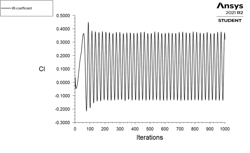
The coefficient of lift = 0.31851738
5. Velocity Contour
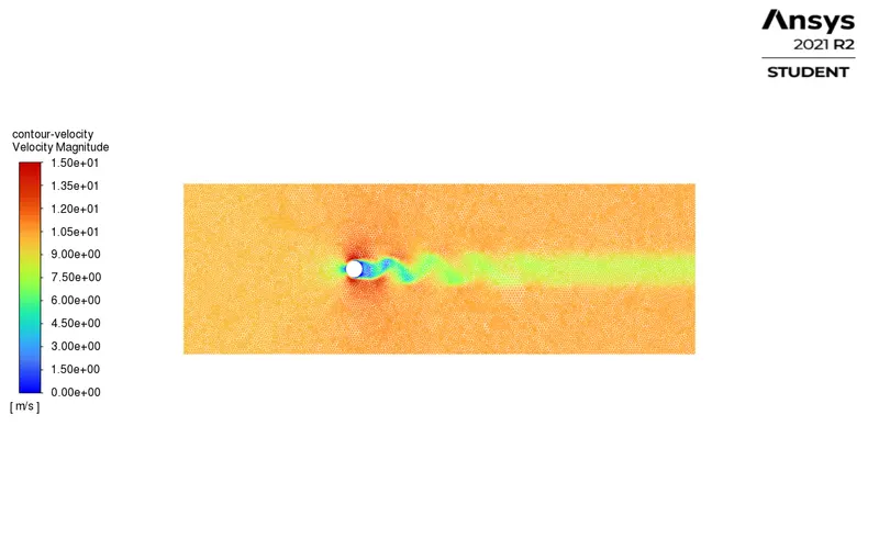
6. Pressure contour
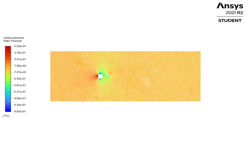
3. Re = 10000
Diameter D = `2m`
Density `rho = 1kg//m^3`
Viscosity `mu=0.02kg//ms`
Reynolds number `Re = 10000`
Velocity `u=(Re*mu)/(rhoD) = 100m//s`
Number of iterations = 1000
- Solutions
1. Residual Plot
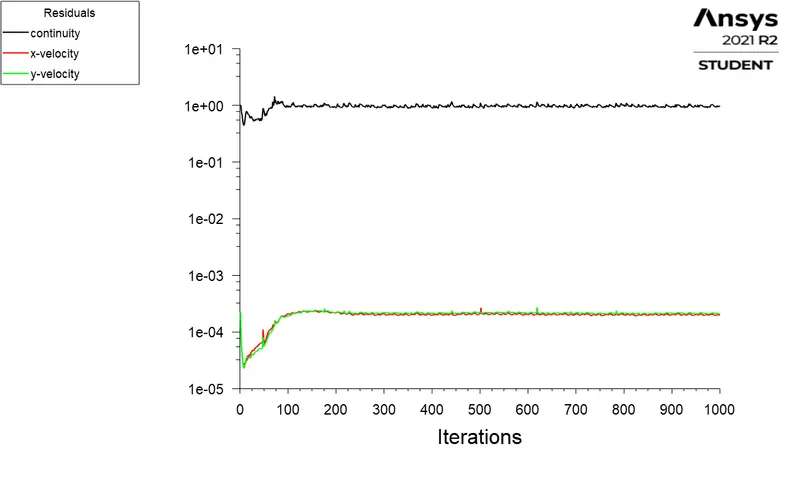
2. Velocity at the monitor point
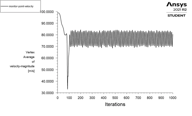
From the above plot, we can say that after some iterations the velocity at the monitor point has been converged. It is also noted that the velocity is oscillating. This can be further understood in contour plots.
3. Coefficient of drag
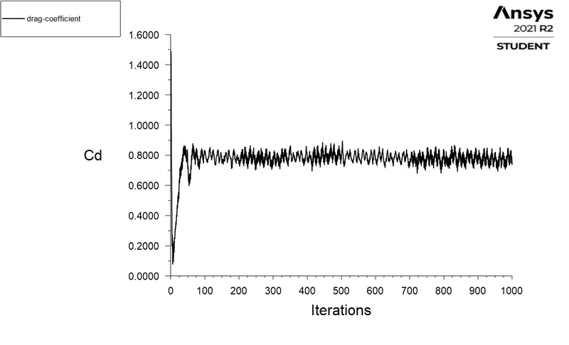
The coefficient of drag = 0.73663974
4. Coefficient of lift
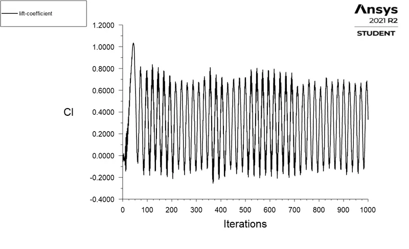
The coefficient of lift = 0.32995503
5. Velocity contour
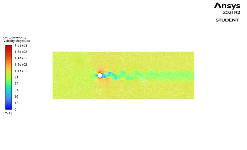
The Velocity contour shows that there is vortex shedding behind the cylinder.
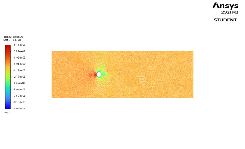
6. Pressure contour
4. Re = 100000
Diameter D = `2m`
Density `rho = 1kg//m^3`
Viscosity `mu=0.02kg//ms`
Reynolds number `Re = 100000`
Velocity `u=(Re*mu)/(rhoD) = 1000m//s`
Number of iterations = 1000
- Solutions
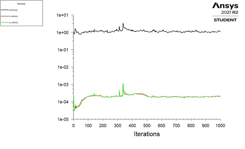
1. Residual plot
2. Velocity at the monitor point
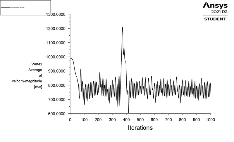
From the above plot, we can say that after some iterations the velocity at the monitor point has been converged. It is also noted that the velocity is oscillating. This can be further understood in contour plots.
3. Coefficient of drag
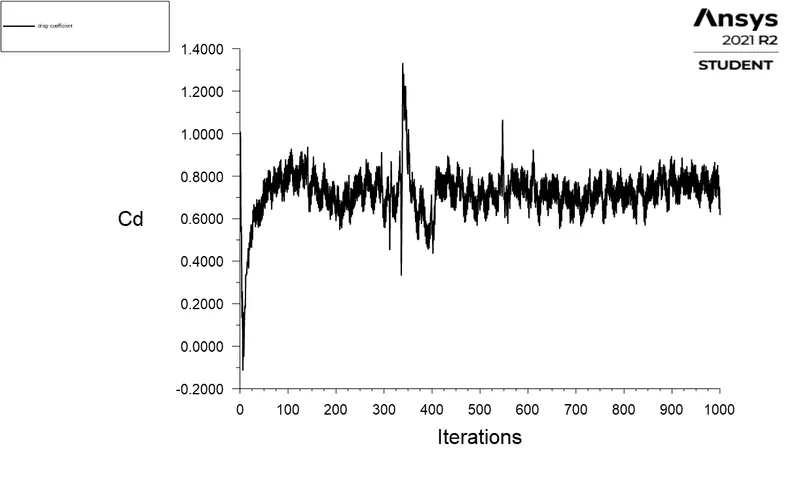
The coefficient of drag = 0.61761727
4. Coefficient of Lift
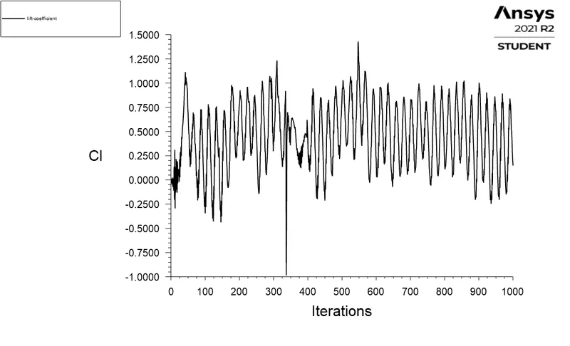
The coefficient of lift = 0.14834287
5. Velocity contour
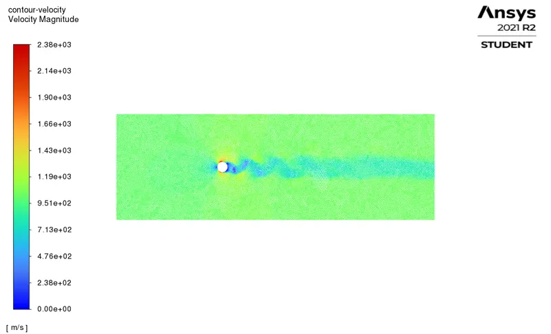
The Velocity contour shows that there is vortex shedding behind the cylinder.
6. Pressure contour
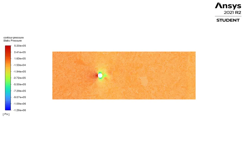
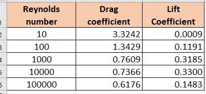
Table - Drag and Lift coefficients at different Reynolds number
Conclusions
- From the steady and unsteady flow over a cylinder at Re =100, we can observe the phenomenon of von Karman Vortex Street behind the cylinder. it is also observed that the velocity at the monitor point is making an oscillating motion which further justifies this phenomenon along with the velocity contour plot.
- The simulation using the steady-state solver arrives at the solution very fast as it is time-independent.
- The steady and unsteady simulation ended up with same results but with the help of time domains in unsteady strouhal number has been captured.
- As the lift coefficient is fluctuating within a limit, a Fourier transformation is carried out to convert the lift values in the time domain to its frequency domain and Strouhal number has been found out.
- The effect of Reynolds number on the flow properties has been studied in the next part by changing the inlet velocity and keeping the fluid same.
- The study shows that at Re=10 there is no formation of vortices behind the cylinder. As the Reynolds number moved past 100 the flow started to separate and a vortex street has been formed behind the cylinder.
- Another important observation is that when the Reynolds number is low, the coefficient of drag is very high. As the Reynolds number increases the drag coefficient got reduced. The above-mentioned table gives a clear picture of this statement.