WEEK 2 - FLOW OVER A CYLINDER.

STEADY & TRANSIENT STATE SIMULATION OF FLOW OVER A CYLINDER IN 2D TO STUDY THE KARMAN VORTEX STREET AND BEHAVIOUR OF CO-EFFICIENT OF LIFT & DRAG USING ANSYS FLUENT

1. AIM:

Our aim is to simulate a steady & transient state flow over a cylinder with different Reynolds number to study the Karman Vortex Street and behaviour of coefficient of lift and drag using the suitable turbulence model using ANSYS FLUENT and validate the numerical result.

2. THEORY/EQUATIONS/FORMULAE USED:

ANSYS FLUENT academic version CFD package is used to carry out the simulation. It is a user-friendly interface which provides high productivity and easy-to-use workflows. Workbench contains all workflow needed for solving a problem such as pre-processing, solving and post-processing.

• Structure of ANSYS FLUENT simulations

The basic steps for a simulation are as follows,

1. Pre-processing – It includes geometry creation, discretization, providing named selection for using as boundary conditions. The packages used in pre-processing step are Space Claim, Ansys Mesher.
2. Solving – It includes applying initial and boundary conditions, adding material properties, applying suitable turbulence model as per the problem and running the iteration till convergence. The package used in post-processing step is Fluent.
3. Post-processing – It includes analysing the results by plotting the results as charts, contour, and exporting the data, also validating the results both qualitatively and quantitatively. The package used in post-processing step is CFD-Post.

KARMAN VORTEX STREET:

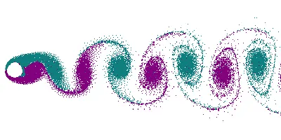
Flow over a cylinder/ blunt body has different patterns depending on the velocity of the flow. As we increase the velocity (Around Reynolds number, Re ≈ 100) oscillating wakes starts forming in the rear end as the momentum of the flow doesn’t allow the flow to surround the object or wrap the contour. The wakes are big enough and are not stable. These wakes from both top and bottom of the rear end of cylinder detaches from the body alternatively. This alternate detachment leads to repeating pattern of swirling vortices called as Karman vortex shedding. It is actually oscillating flow pattern observed in a flow past a blunt body as shown the figure above.

Strouhal Number:

It is the ratio of inertial forces due to the local acceleration of the flow (unsteadiness of the flow) to the inertial forces due to the convective acceleration (change in velocity from one point to another point). In simple words we can say that it is ratio of oscillation to the velocity.

St = (f * L )/U where f = vortex shedding frequency, L = characteristic length, U = Flow velocity

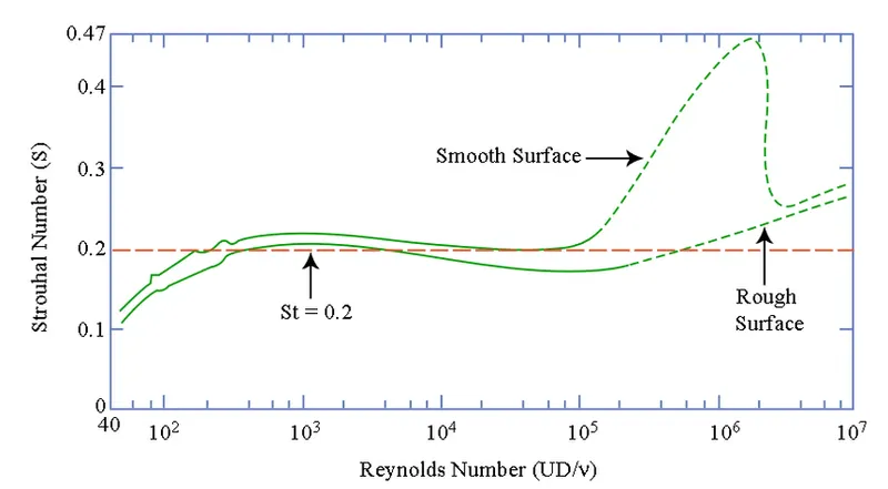
It is actually used in order to study the oscillating flow mechanism, a dimensionless number which describes the flow fluctuations or instabilities. Strouhal number is calculated to study the velocity fluctuations in the region of Karman vortex shedding, also to describe flapping wing flight. This parameter is named after Vincenc Strouhal, a Czech physicist. In general, Strouhal number ranges from 0.12 to 0.30. Basically, high Strouhal number means the oscillation dominates the flow and low Strouhal number means the flow speed over rules the oscillations.

Fast Fourier Transform (FFT):

Fourier transform is basically done to convert a sequence of signals in the time domain into a frequency domain. FFT is used instead of Discrete Fourier transform (DFT) is because FFT is more efficient and fast comparatively which reduces the computation time.

Reynolds Number:

It is a ratio of inertial force to the viscous force. It is a dimensionless number used to categorize any fluid where viscosity plays an important role, as viscosity controls the velocity.

Reynolds Number = Inertial Force / Viscous Force

Re = (ρ * u * L) / µ

where Re is Reynolds number, ρ is Density of the fluid, L is Length of the pipe, u is flow speed and µ is Dynamic Viscosity of the fluid.

The dimensionless number is used to determine if a fluid is laminar or turbulent. Assumed criteria for Reynolds number are as follows:

1. Internal flow:

Re ≤ 2100 is laminar flow.

Re ≥ 2100 and ≤ 4000 is Critical flow.

Re ≥ 4000 is turbulent flow.

2. External flow:

Re ≤ 100000 is laminar flow.

Re ≥ 100000 and ≤ 500000 is Critical flow.

Re ≥ 500000 is turbulent flow.

Why there is a difference in criteria between Internal and external flows?

In external flow, the viscous boundary layer region grows along the length of the surface. So Reynolds number is calculated by using Re = (ρ * u * L)/ µ , where Re is Reynolds number, ρ is Density of the fluid, L is Length of the pipe, u is flow speed and µ is Dynamic Viscosity of the fluid.

In internal flows, the viscous boundary layer region of all surface merges together into fully developed flow and the grows around the width of the surface. Hence, Reynolds number is calculated by using Re = (ρ * u * W)/ µ , where Re is Reynolds number, ρ is Density of the fluid, W is width of the pipe, u is flow speed and µ is Dynamic Viscosity of the fluid.

Hence, in external and internal flow the Reynolds number is based on length along the flow and thickness across the flow respectively.

In case the Reynolds number is calculated for external flow with known value of boundary layer thickness then it will become equal as that of internal flow.

Re_δ = (ρ * u * δ)/ µ ,

where Re is Reynolds number, ρ is Density of the fluid, δ is boundary layer thickness, u is flow speed and µ is Dynamic Viscosity of the fluid.

Coefficient of Lift

Lift Force = ½ ρ V²C_l A

Flow over a cylinder is expected to have a fluctuation in velocity at Reynolds number around 100. These fluctuations are captured in terms of coefficient of lift in time domain and then Strouhal number is determined by using Fourier transform.

Coefficient of Drag

Drag Force = ½ ρ V²C_d A

where ρ is Density of the fluid, A is surface area, V is flow speed and C_l & C_d are Coefficient of Lift and Coefficient of Drag respectively.

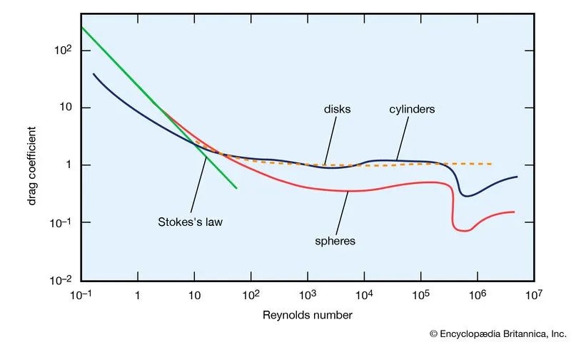
Behaviour of Coefficient of Drag at varying Reynolds Number

Two factors responsible for total drag are viscous drag (skin-friction drag) and form drag (Pressure drag/ Profile Drag). Coefficient of Drag is function of Reynolds number, shape along with other factors.

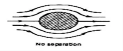
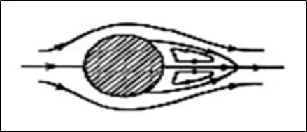
Flow over a cylinder/ blunt body has different patterns depending on the velocity of the flow.

1. Creeping Flow - No Separation:

2. Steady Boundary Layer Separation:

3. Karman Vortex Shedding:

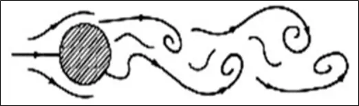
4. Turbulent Wakes:

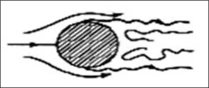
5. Turbulent Boundary Layer:

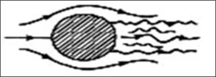
As we increase the velocity (Around Reynolds number, Re ≈ 105 – 106) boundary layer becomes turbulent and flow wraps around the object, now highly resistant to separate. So, the flow stays attached longer resulting in compression (narrow) of turbulent wakes. This case is somewhat similar to case 2 but as the skin-friction drag is very negligible and also the form drag is less than the previous case 4 the coefficient of drag drops drastically known as drag crisis. But again, Cd rises and level off and then probably decline again.

Problem – Flow over a Cylinder:

The challenge includes 2 parts.

• Steady and transient state simulation of flow over a cylinder of dia. 2m in 2D and to determine the Strouhal number for Reynolds number, Re = 100.
• Calculate the coefficient of Drag and Lift over a cylinder at different Re = 10, 100, 1000, 10000, 100000 with steady state solver and to study its effect on coefficient of drag.

Calculation:

Reference values (common for Part 1 and Part 2)

Length = 2 m (Dia. of the cylinder), Depth = 1m (2D)

Area = Length x Depth = 2 m²

Part 1 - Steady and Transient State

Customized fluid is created by changing the density and dynamic viscosity of the fluid in order to make Reynolds number exactly 100 and calculation easier.

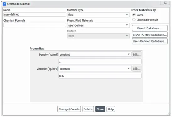
Fluid chosen for the problem – User Defined

Density of Air = 1kg/m3, Dynamic viscosity = 0.02 kg/ms, Velocity of fluid = 1 m/s, Characteristic length = 2 m

So, Reynolds Number, Re = 100

Transient State

Courant- Friedrichs-Lewy condition is followed to determine the time step,

CFL = u*(Δt/ Δx), where u = velocity, Δt = time step, Δt = cell size.

So for CFL = 0.4, Velocity, u = 1 m/s, Cell size, Δx = 0.5 m

Time step, Δt = 0.2 s

Part 2 - Steady State

Coefficient of lift and drag needs to be calculated for different Reynolds number, so velocity differs for each setting of Reynolds number.

Fluid chosen for the problem – Air

Density of Air = 1.225 kg/m3, Dynamic viscosity = 1.7894 x 10-5 kg/ms, Characteristic length = 2 m

For Re = 10, V = 0.000073 m/s

For Re = 100, V = 0.00073 m/s

For Re = 1000, V = 0.0073 m/s

For Re = 10000, V = 0.073 m/s

For Re = 100000, V = 0.73 m/s

PROCEDURE

Part 1:

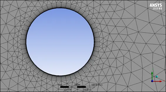
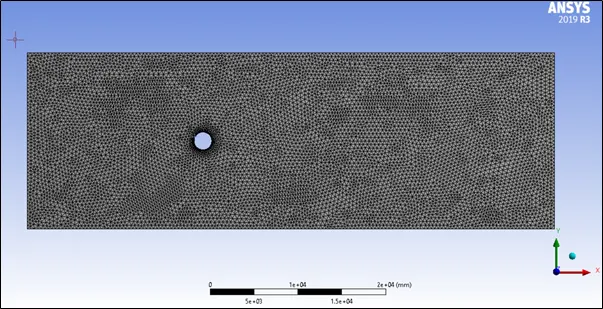
• In the process, firstly the geometry with flow domain is created in SpaceClaim. Then the meshing is done in order to study the flow near the walls clearly and named the boundaries. Also made sure that mesh is good enough to carry out the current simulation.
• In fluent, the user-defined material, solver type, the initial and boundary condition, suitable turbulence model are defined as per the problem.
• Monitor points are created in order to study the velocity fluctuation and pressure, velocity contours are created to monitor during run time.
• Coefficient of lift plot is also initiated in order to use for Strouhal number calculation by fast Fourier transform method. Finally the animation is also added to study the overall behavior after the simulation is converged.

Part 2:

• The geometry with flow domain and mesh remain common for both part 1 and part 2. In fluent, the fluid chosen for simulation is air.
• The solver type, the initial and boundary condition, suitable turbulence model are defined as per the problem.
• Monitor points are created in order to study the velocity fluctuation and pressure, velocity contours are created to monitor during run time.
• Coefficient of lift and drag plot is also set in order to study the effects. Finally the animation is also added to study the overall behavior after the simulation is converged.
• The same procedure is followed for each simulations with Reynolds number equal to 10, 100, 1000, 10000, 100000.

NUMERICAL ANALYSIS (Software used – ANSYS 2020 R2)

Geometric Model

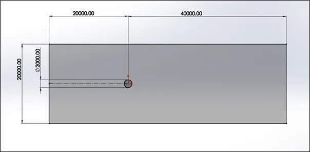
The 2D geometry of cylinder (D = 2m) with flow domain is created in Space Claim as per the figure given below. In order to study the external flow behaviour, the domain width of 10D is created. Also, a space of 10D before the cylinder and more importantly 20D after the cylinder is created to capture the flow.

2D Geometry with the flow domain – Flow over a Cylinder

Mesh Generation:

Solver Set-up:

• The mesh file is imported into the FLUENT software for the analysis of the modelled surface.
• Once the mesh file is loaded and displayed, it is checked for the units, scale, and mesh.
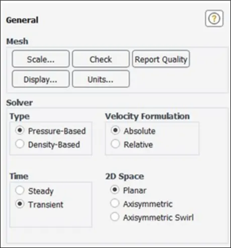
• There are two types of numerical solver methods pressure –based and density-based solver. The pressure-based solver was used rather than the density-based solver as the simulation is for lower Mach number. Absolute velocity formulation, steady and transient state was used for the analysis.

• Energy equation was switched off for the analysis process as we are not interested in temperature of the system.
• Laminar turbulence model was used for the analysis as the Reynolds number used for simulation is in the range of 10 to 100000.

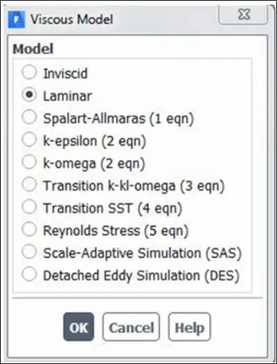
• The fluid material chosen for part -1 is user defined and for part-2 is air.

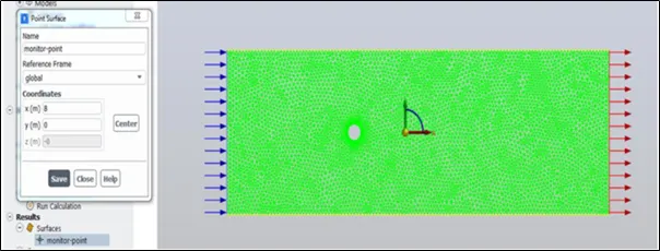
• Monitor point are created at 8m from the centre of the cylinder to observe the velocity fluctuations.

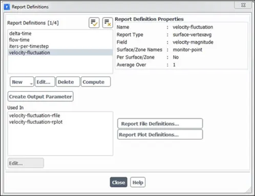
• Report definitions such as vertex average for velocity at the monitor points, Coefficient of Lift and Drag of are set up as we are interested in the physical quantity such as velocity fluctuation at the monitor point, coefficient of lift and drag.

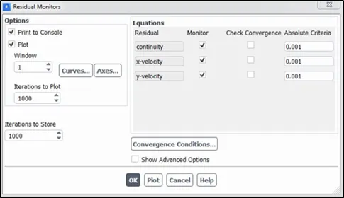
• Convergence Criteria are left unchecked as it might take some more time and we want to run the complete number of iterations or time step set for the simulation in order to witness the physics behind of the problem.

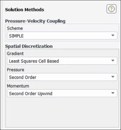
• Solution methods – SIMPLE Scheme used for Pressure-Velocity coupling and the methods for Spatial Discretization are as per the below image.

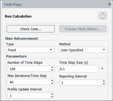
• Hybrid initialization is done and numbers of iterations are set for running the steady simulation and time step size and number of time step for transient simulation.

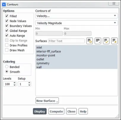
• Velocity and pressure contours are set in order to monitor the fluctuations during run time and also animations are added.

Initial Setup and Boundary Condition:

Part – 1

Zone	Type	Boundary Condition	Additional conditions (if any)
Inlet	Velocity - Inlet	Velocity – 1 m/s,	Steady State, Transient State, Pressure Based, Absolute Switched OFF Energy equation Turbulence Model – Laminar
Outlet	Pressure - Outlet	Gauge pressure of 0 Pa
Symmetry	Symmetry	Symmetry
Walls	Wall	Stationary wall without slip

Note - Coefficient of lift plot at wall is created in order to calculate the Strouhal number using Fast Fourier Transform.

Part – 2

Zone	Type	Boundary Condition		Additional conditions (if any)
Inlet	Velocity - Inlet	Reynolds Number	Velocity, m/s	Steady State, Pressure Based, Absolute Switched OFF Energy equation Turbulence Model – Laminar
		10	0.000073
		100	0.00073
		1000	0.0073
		10000	0.073
		100000	0.73
Outlet	Pressure - Outlet	Gauge pressure of 0Pa
Symmetry	Symmetry	Symmetry
Walls	Wall	Stationary wall without slip

Note - Coefficient of drag plot at wall is created in order to study the effect of Reynolds Number.

RESULTS:

Part – 1 @ Re = 100

Steady State:

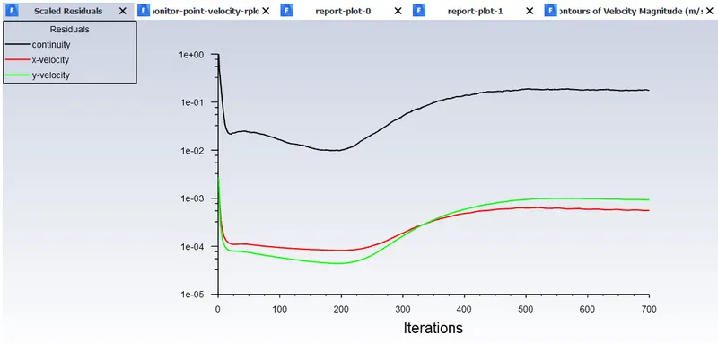
• Convergence Plot

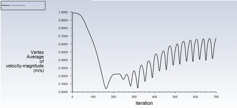
• Velocity Fluctuation at monitor point

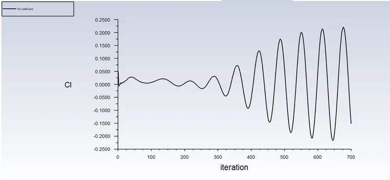
• Coefficient of Lift plot at wall

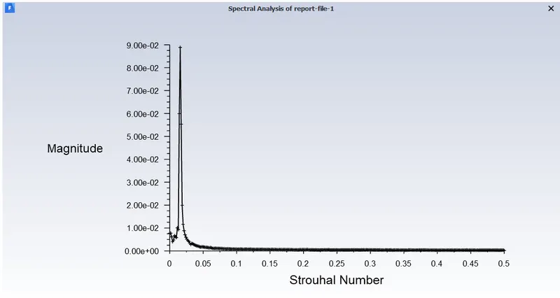
• Strouhal Number Plot

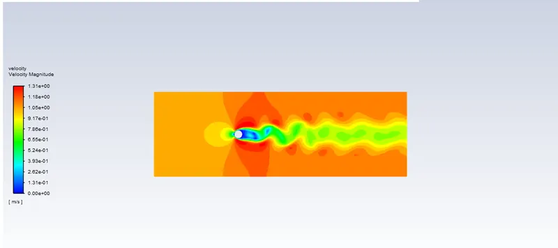
• Velocity contour of flow over a cylinder

Transient State:

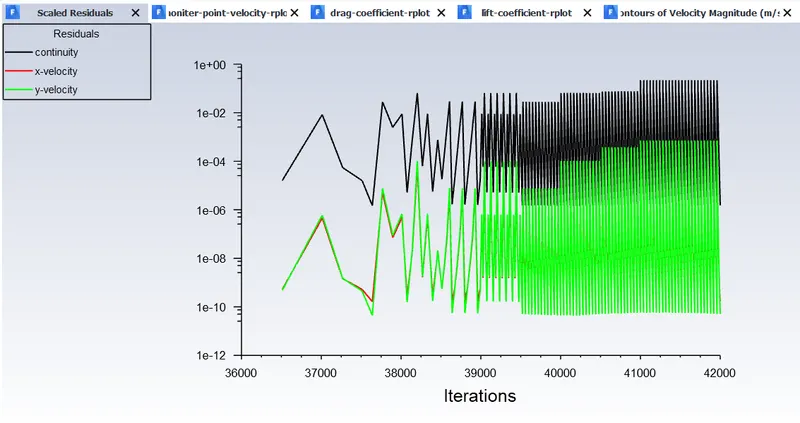
• Convergence Plot

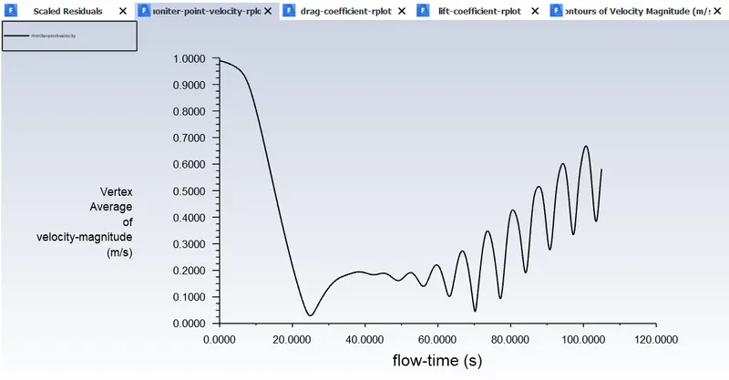
• Velocity Fluctuation at monitor point

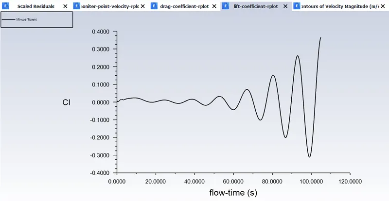
• Coefficient of Lift plot at wall

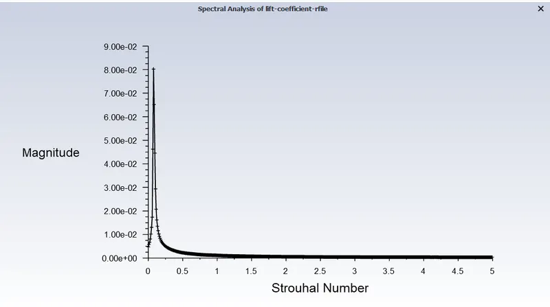
• Strouhal Number Plot

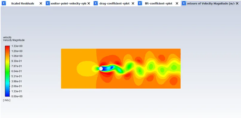
• Velocity contour of flow over a cylinder

Conclusion

Part 1

1. The steady-state and transient state simulation is done for studying the laminar flow past the cylinder, velocity fluctuations with user-defined material in order to solve exactly at Reynolds number equal to 100 in ANSYS FLUENT.
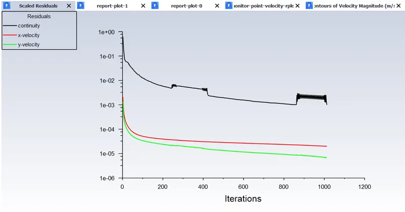
2. From the convergence plot we can see that in steady state, the solution is converged after 200 iterations but in transient state the convergence plot is fluctuating.
3. Also the average velocity at the monitor point shows oscillations in both steady and transient simulations.
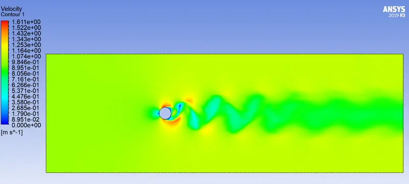
4. Velocity and Pressure contour clearly shows the oscillating wakes getting detached from the top and bottom of the rear end alternatively at Reynolds number = 100. This is known as Karman vortex shedding.
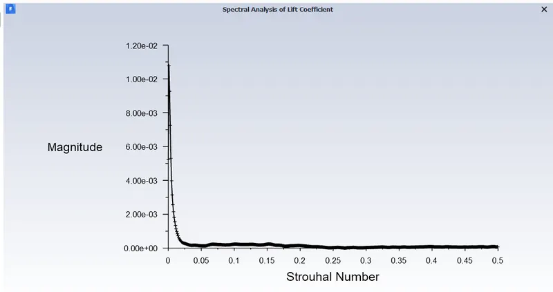
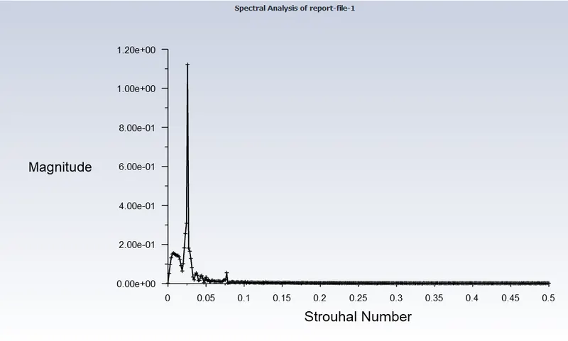
5. Coefficient of lift plot obtained in transient state simulation is used calculate the Strouhal number as its time dependent.
6. Strouhal Number = 0.15 is determined using Fast Fourier transform (FFT) to convert the time domain results into frequency domain.
7. As theoretical concept suggests, we could see Karman vortex shedding in laminar flow starting at Reynolds Number = 100 and the corresponding Strouhal Number in the range of 0.15-0.16. Hence the results are in good agreement and the underlying physics is visible clearly.

Part – 2 - Steady State

• Convergence Plot

Re - 10

Re - 1000

Re - 10000

Re - 100000

• Velocity Fluctuation at monitor point

Re - 10

Re - 1000

Re - 10000

Re - 100000

• Coefficient of Lift plot at wall

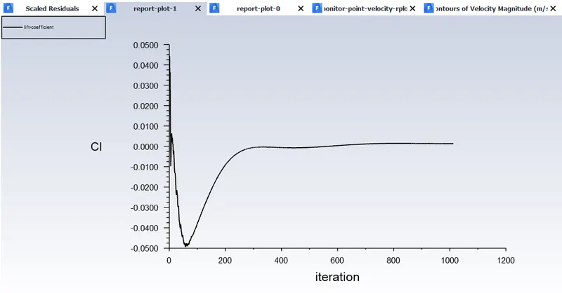
Re - 10

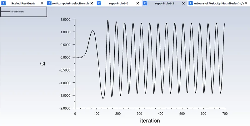
Re - 1000

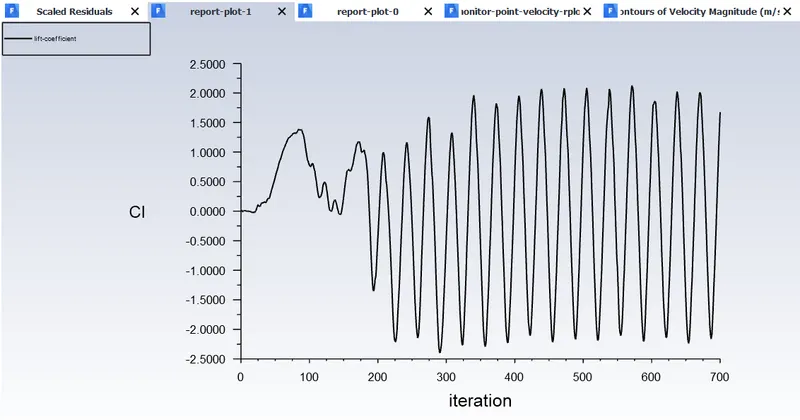
Re - 10000

Re - 100000

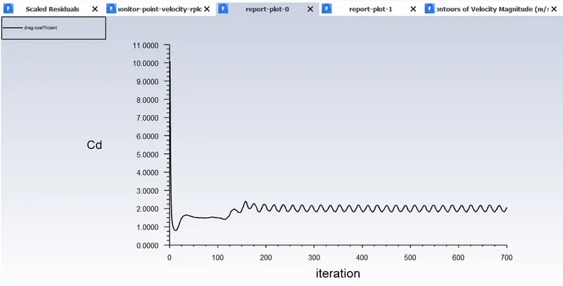
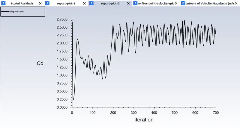
• Coefficient of Drag plot at wall

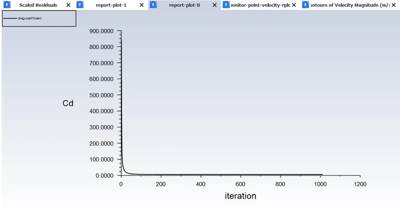
Re - 10

Re - 1000

Re - 10000

Re - 100000

• Strouhal Number Plot

Re - 10

Re - 1000

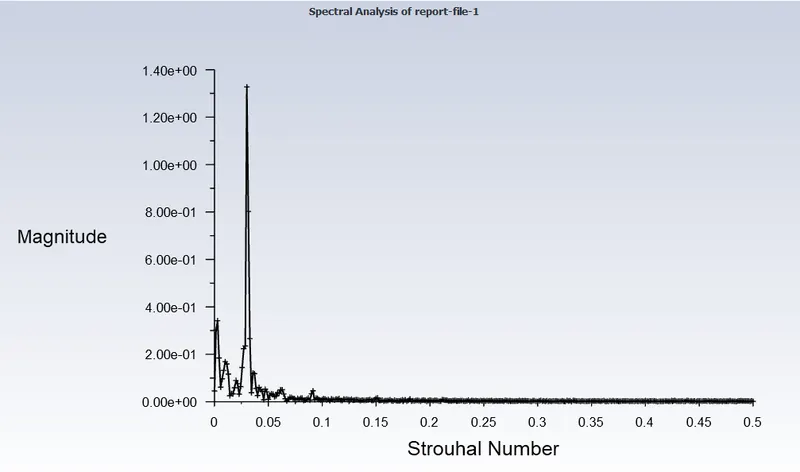
Re - 10000

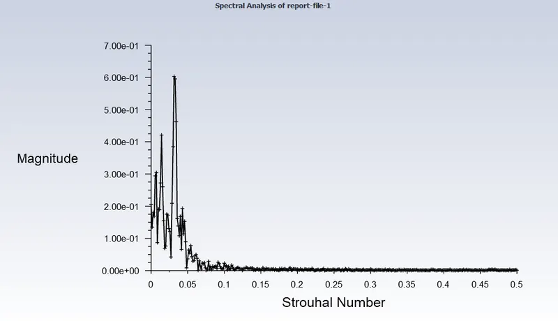
Re - 100000

• Velocity contour of flow over a cylinder

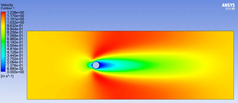
Re - 10

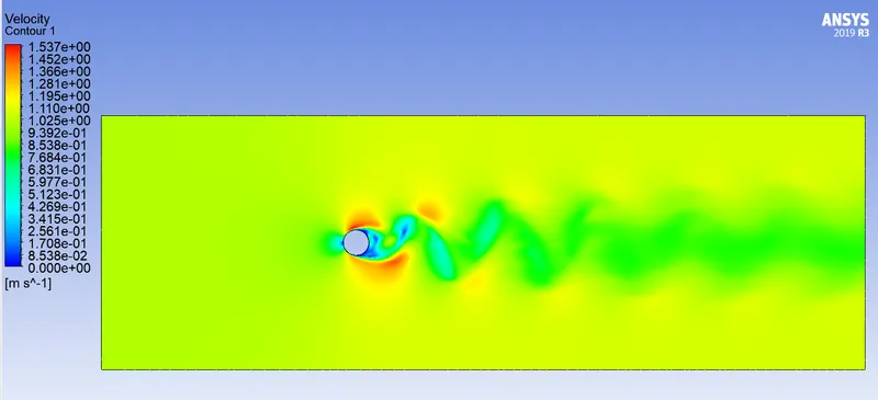
Re - 1000

Re - 10000

Re - 100000

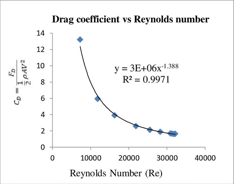
Effect of Reynolds number on Coefficient of Drag and Lift

Sr. No.	Reynolds Number	Cd	Cl
1	10	3.3181835	0.000816789
2	100	1.3261365	0.106640060
3	1000	1.0530861	- 0.041658008
4	10000	1.0829977	- 0.236503880
5	100000	0.8352106	- 0.351732790

CONCLUSION (PART – 2)

1. The steady state flow over a cylinder is solved to calculate the coefficient of lift and drag at Reynolds number equals to 10, 100, 1000, 10000, 100000 and study the effect of Reynolds number on coefficient of drag.
2. Laminar turbulence model was used for all the 5 cases with air as the chosen fluid for the simulation.
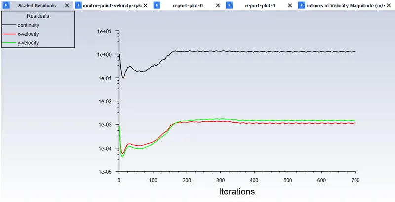
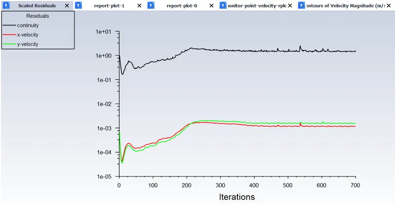
3. From the convergence plot we can see that, the solution is getting converged faster as the Reynolds number is increasing. As the convergence factor is unchecked but we can still see the steady pattern is followed after a certain number of iteration which can be considered as solution convergence.
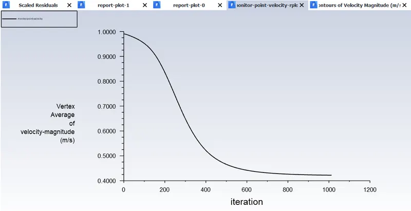
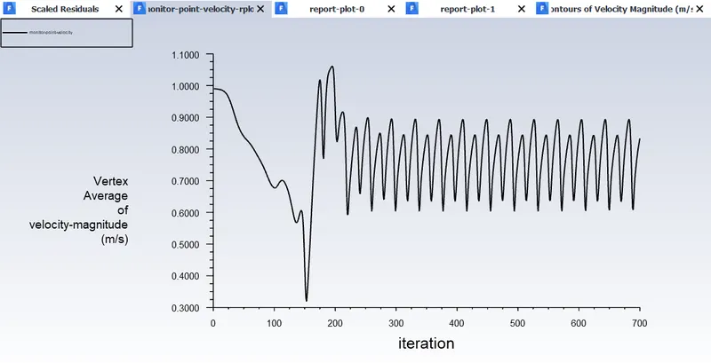
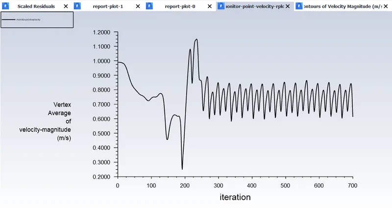
4. The average velocity plot at the monitor point shows oscillations starting from Reynolds number 100 and keeps growing till the Reynolds number 100000.
5. The velocity and pressure contour clearly shows the oscillating wakes getting detached from the top and bottom of the rear end alternatively starting at Reynolds number = 100.
6. As theoretical concept suggests, the Coefficient of Drag reduces as the Reynolds number increases as shown in the above graph. Hence the results are in good agreement and the underlying physics is visible clearly.