Week 2 - Flow over a Cylinder.

AIM:

To simulate the flow over a cylinder and understand the Von Karman Vortex street phenomenon using ANSYS software.

OBJECTIVE:

• To simulate the flow with the steady and unsteady case and calculate the Strouhal Number(Sr) for Re= 100.
• To calculate the coefficient of drag`(C_d)` and lift`(C_L)` over a cylinder by setting the Reynolds number to 10,100,1000,10000 & 100000 using steady state solver.
• To discuss the effect of Reynold's number on the coefficient of drag and validate the results with the standard literature.

INTRODUCTION - FLOW OVER A CYLINDER:

• Simulation of flow over a cylinder is a very important problem in fluid mechanics because of its complex unsteady dynamics of the cylinder wake flow. The laminar vortex shedding known as "Von Karman vortex street" takes place at Reynold's number greater than 40.
• The frequency of vortex can affect the cylinder if this frequency is closer to the structural natural frequency of the cylindrical body causing resonance.
• Hence, Vortex shedding phenomenon is of great interest in the field of Automobiles, Aerospace, Renewable energy, Constructions etc..Therefore, understanding the flow behind the cylinder plays a crucial role in these industries in the stage of Computer aided Engineering.

Von Karman Vortex shedding:

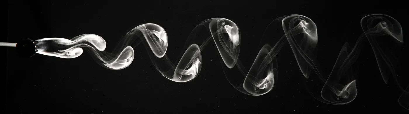
• In fluid dynamics, a Kármán vortex street (or a von Kármán vortex street) is a repeating pattern of swirling vortices, caused by a process known as vortex shedding, which is responsible for the unsteady separation of flow of a fluid around blunt bodies.
• A term defining the periodic detachment of pairs of alternate vortices from a bluff-body immersed in a fluid flow, generating an oscillating wake, or vortex street, behind it, and causing fluctuating forces to be experienced by the object.
• The phenomenon was first observed and analyzed on two-dimensional cylinders in a perpendicular uniform flow, but it is now widely documented for three-dimensional bodies and non-uniform flow fields.
• This is a situation where the energy subtracted from the flow field by the body drag is not dissipated directly into an irregular motion in the wake, but it is first transferred to a very regular vortex motion. The structure of the flow is then as schematically indicated;

• "Karman Vortex street" is the phenomenon which takes place behind a bluff body at Reynold's number greater then 40 at which the wake behind the cylinder becomes unstable.
• This wake develops a slow oscillation with loss of flow symmetry and vortices are shed from the cylinder surface. The ampitude of the oscillation increase in downstream direction.
• This phenomenon is shown in the image given below;

• A dimensionless number 'Strouhal number `(S_r)`' is used to analyze the oscillating unsteady fluid flow dynamics problems. It represents the radio of inertial forces due to the unsteadiness of the flow or local acceleration to the inertial forces due to changes in velocity from one point to another in the flow field.

ROLE OF DIMENSIONLESS NUMBERS IN THIS PROJECT:

• Reynolds number , `Re = (vD)/nu`=`(rho vD)/mu`

Where `v` is the flow velocity , `D` is the characteristic length of the geometry and `nu` is the kinematic viscosity of the fluid.

• Drag coefficient , `C_d=(2F_d)/(rhov^2A)`

Where `F_d` is the drag force , `rho` is the density of the fluid , `v` is the flow velocity and `A` is the cross sectional area.

• Lift coefficient , `C_L=(2F_L)/(rhov^2A)`

Where `F_L` is the lift force , `rho` is the density of the fluid , `v` is the flow velocity and `A` is the cross sectional area.

• Strouhal number , `Sr = (fL)/v`

Where `f` is the frequency of the vortex shedding , `L` is the characteristic length and `v` is the flow velocity.

PROCEDURE

GEOMETRY:-

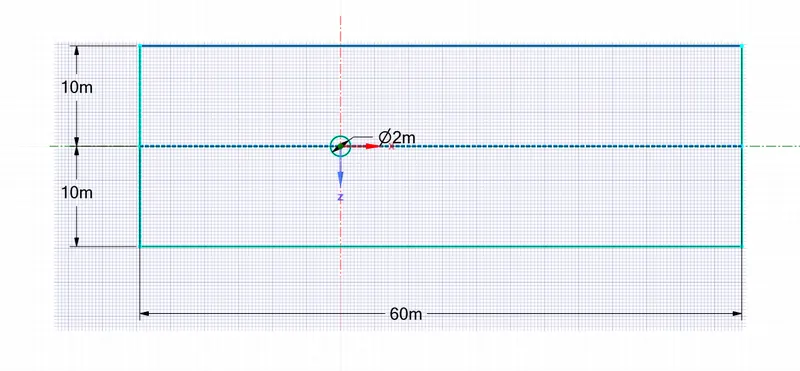
• The 2D geometry with the following dimensions has been constructed by using geometry tools available in ANSYS SpaceClaim.
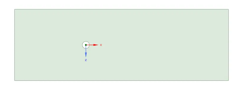
• It consists of a rectangular fluid domain and a cylinder as an obstruction. The feature 'Surface Pull' in SpaceClaim has been utilised to delete the cylinder surface.

MESHING:-

• The Meshing is done using ANSYS Meshing where the triangular mesh is applied for the body by using 'Methods'.
• Element size: 0.25m
• Nodes: 20697
• Elements: 40502

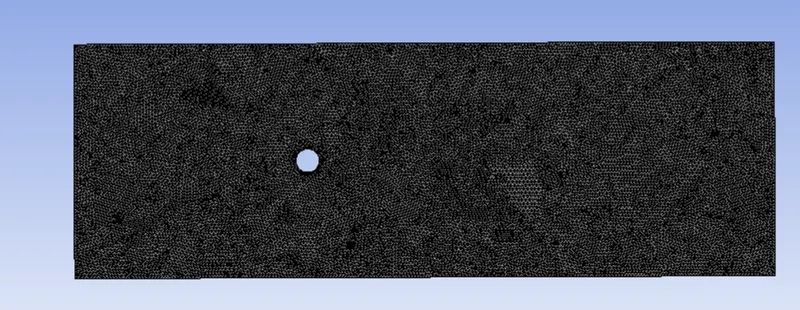
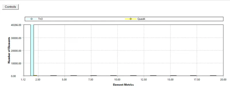
• The Element quality has been shown below which describes that most of the elements have more than 90% quality.

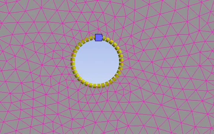
• Using 'Edge sizing' tool the smoothness of the circle edge is improved by setting number of divisions to 36.

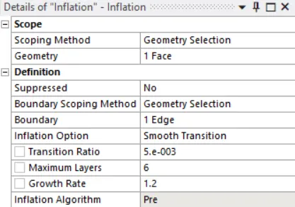
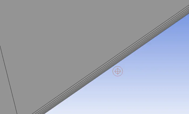
• 'Inflation' option is used to create an inflation layer around the circle for the Body fitted mesh with 6 layers to create high quality geometry to capture the physics near the cylinder wall accurately.

• Then the inlet, outlet, wall and symmetry boundaries are named for this meshed geometry which can be good for fluent setup.

FLUENT SET-UP:

1) Steady and Transient state Simulations at Re=100:

*Set-up for steady state simulation

• 'Check mesh' option is used here to check Mesh statistics and also whether the mesh qualifies on Topology check and Geometry check.
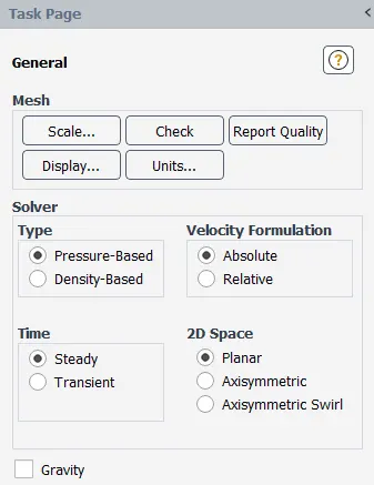
• In the General tab, the following setup has to be set for steady state simualtion.

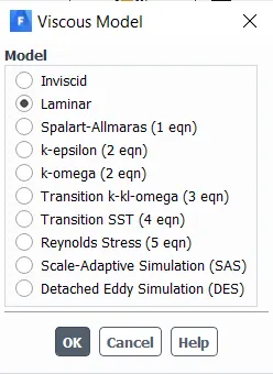
• Viscous model

• Materials : Fluid - Air(user_material)

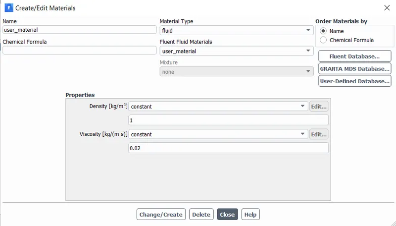
• Where Reynold's number, `Re = (rho.d.u)/(mu) = (1*2*1)/(0.02) = 100`
• Boundary conditions:
  • Inlet: velocity-inlet type, 1 m/s
  • Outlet: pressure-outlet type, zero gauge pressure
  • Cylinder wall: type wall, No slip conditions
  • Symmetry: symmetry type
• Solution methods: SIMPLE (Semi implicit method for pressure linked equations ) for Steady state

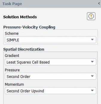
• To analyze the velocity of the flow at the cylinder wake , a monitor point is placed at a distance of 4D (where D is the diameter of the cylinder) which is 8m from the center of the cylinder to behind.

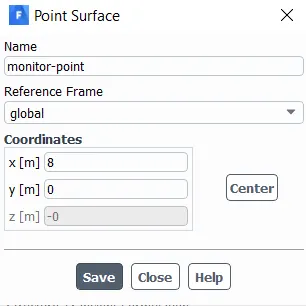
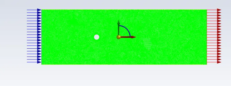
• Then the velocity vertex average at this monitor point is calculated.

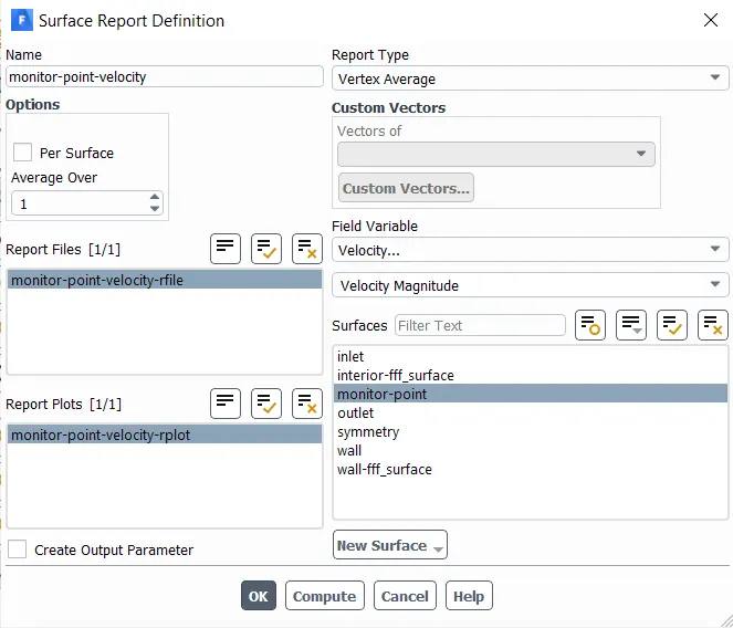
• Initialization: Hybrid, No.of iterations: 700
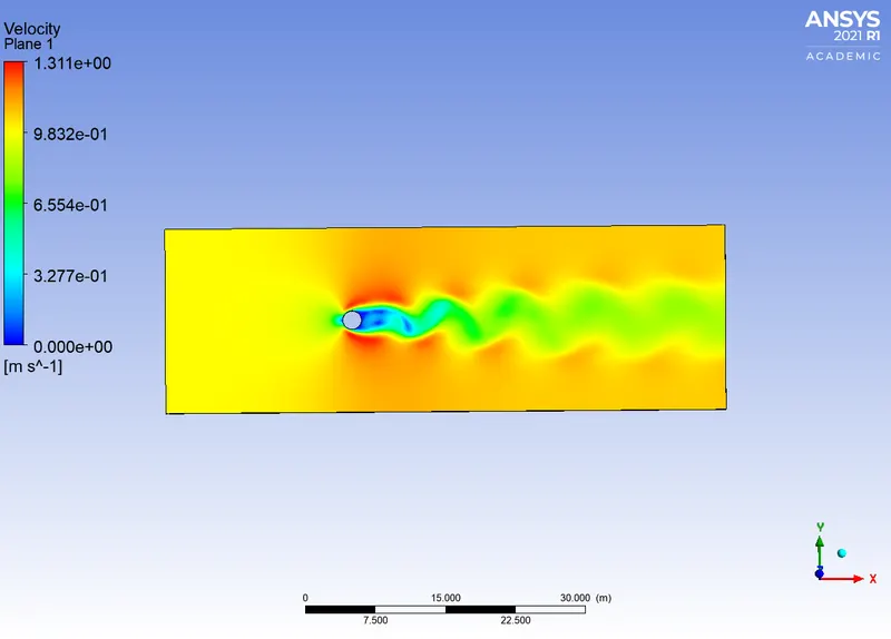
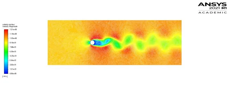
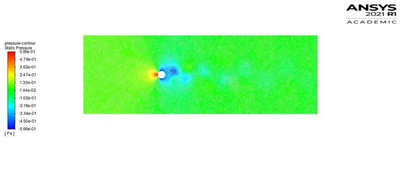
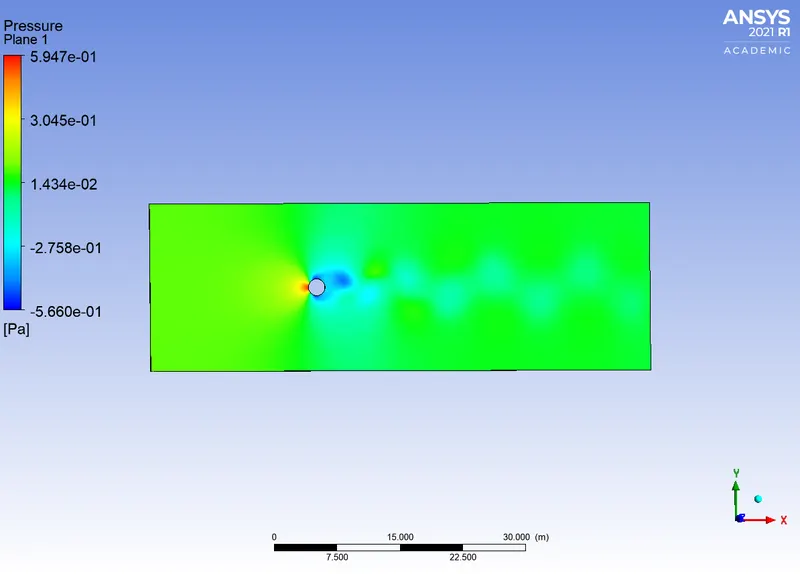
• Velocity and Pressure contours are created to visualize the vortex shedding pheomenon.

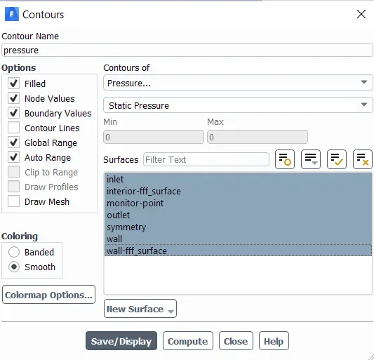
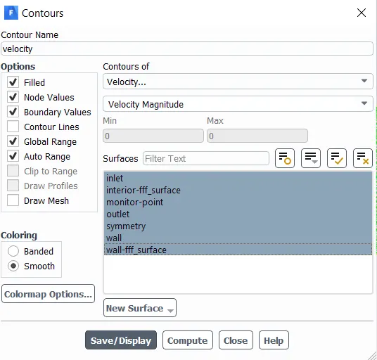
• Solution animation is created from the 'Activities' tab by selecting the contour plots.

*Set-up for Transient state simulation

• Solver time : Transient
• Initialization : Hybrid
• Time step size : 0.1s
• Number of time steps : 1000
• The monitor point is created at a distance of 3D(6m) from the cylinder in the axial direction.

Set-up to calculate the Coefficient of drag and lift:

• Before proceeding to calculate the Coefficient of drag and lift , we have to set the reference values in ANSYS Fluent to compute from the inlet, this is done as shown below;

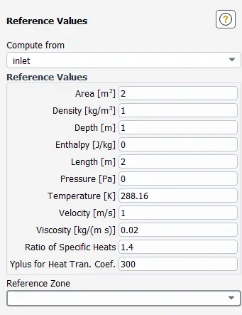
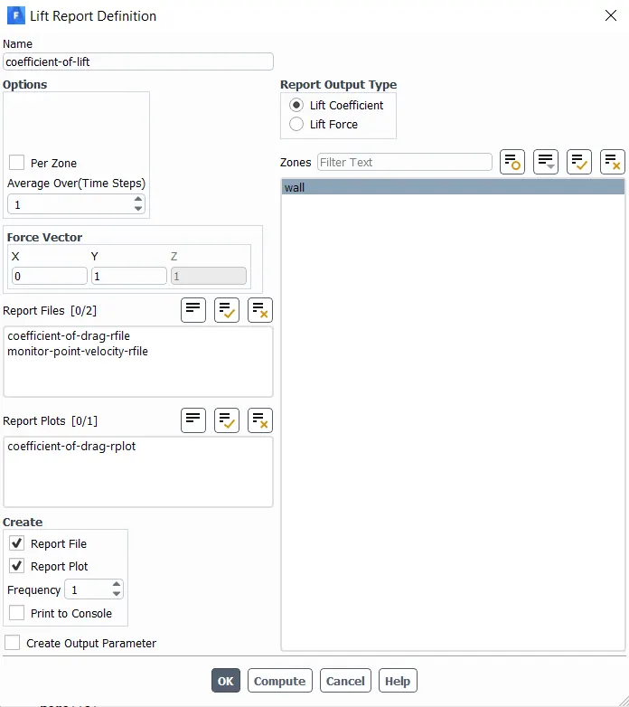
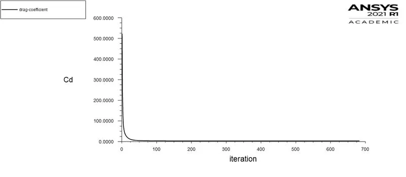
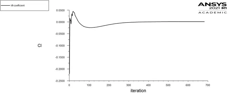
• Then, the drag and lift coefficient's plots are separately created under 'definitions-> Force Report'. This will give the required plots.

Set-up to calculate the Strouhal Number (Sr):

• Strouhal number denoted by 'Sr' is a dimensionless number which is used to describe oscillating flow mechanisms such as vortex shedding.
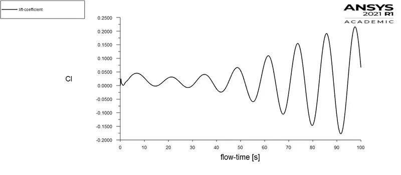
• The Strouhal number is calculated by using the unsteady state simulation results. The coefficient of lift values at each timestep has to be loaded as an input file to calculate the strouhal number.

• A Fourier transform is done mainly to convert a sequence of signals in the time domain to its frequency domain. FFT stands for Fast Fourier Transform, which is a Discrete Fourier Transform that takes in a sequence of values in space/time domain and converts it into a sequence of frequencies.

• The FFT in Ansys fluent enables you to find the frequency of time data by considering a finite number of sampled data points. It uses the Fast Fourier Transform as it is comparatively faster than a direct Fourier transform.

• The Fast Fourier Transform (FFT) is used to find the strouhal number, which will convert the time dependent value of lift coefficient to the frequency domain. On the X-axis ,Strouhal number is selected and on the Y-axis, Magnitude is selected. Then, load the calculated values of lift coefficient using 'Load input file' option. This set-up is shown below,

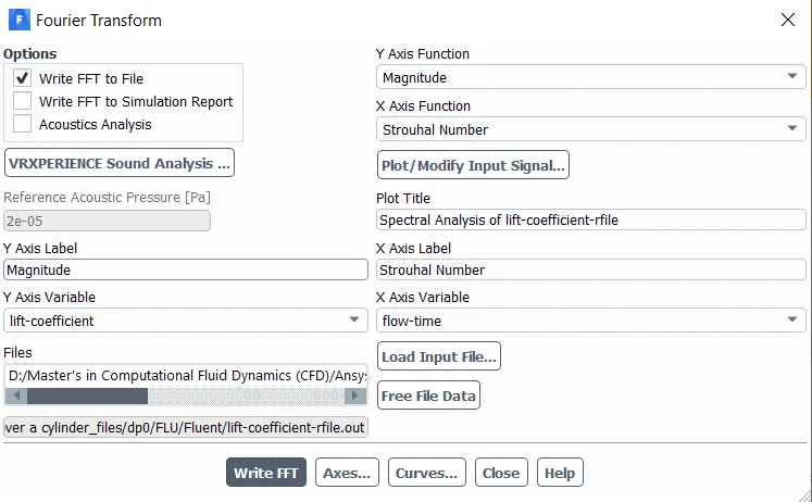
• From the output results of the FFT file which is obtained by clicking on 'write FFT to file', the required Strouhal number will be the one with the highest magnitude value correponding to it.

RESULTS

Steady state simulation at (Re = 100)

Scaled Residuals graph

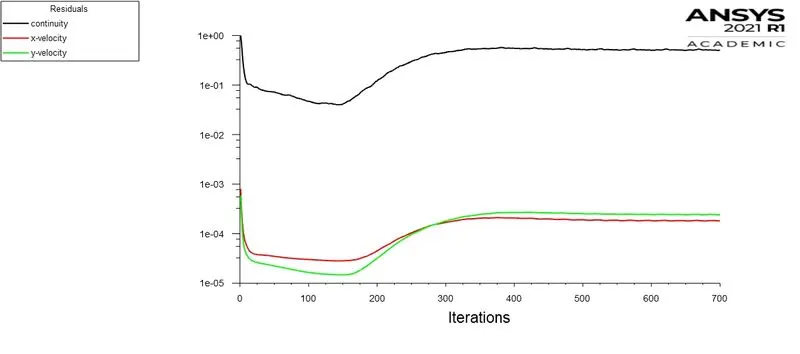
• After around 400 iterations, the residuals doesn't change and gives us constant values.

Vertex average velocity at the monitor point

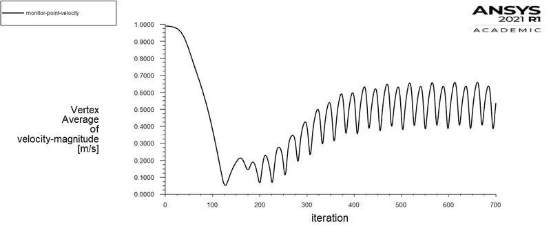
• From the above plot, we can observe that the vertex average of velocity magnitude started to give similar pattern after about 400 iterations.
• By analysing both the residuals graph and vertex average velocity plot, we can conclude that the solution has been converged at around 400 to 500 iterations.

Velocity Contour

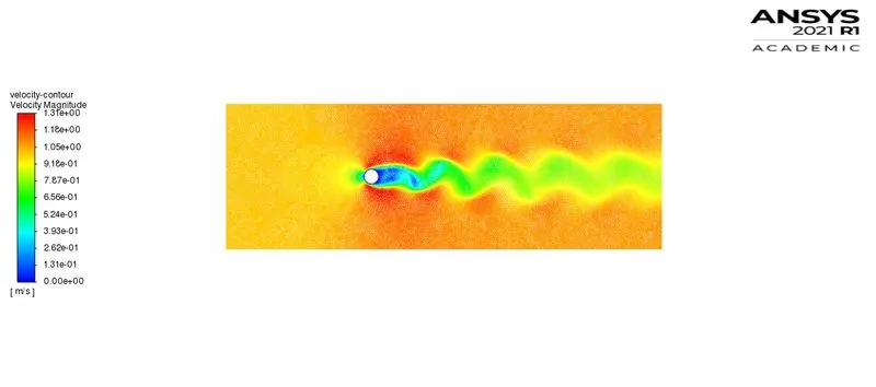
At CFD Post

Pressure Contour

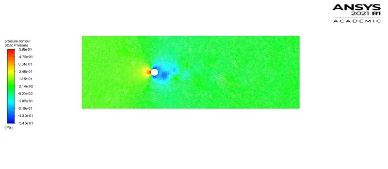
At CFD Post

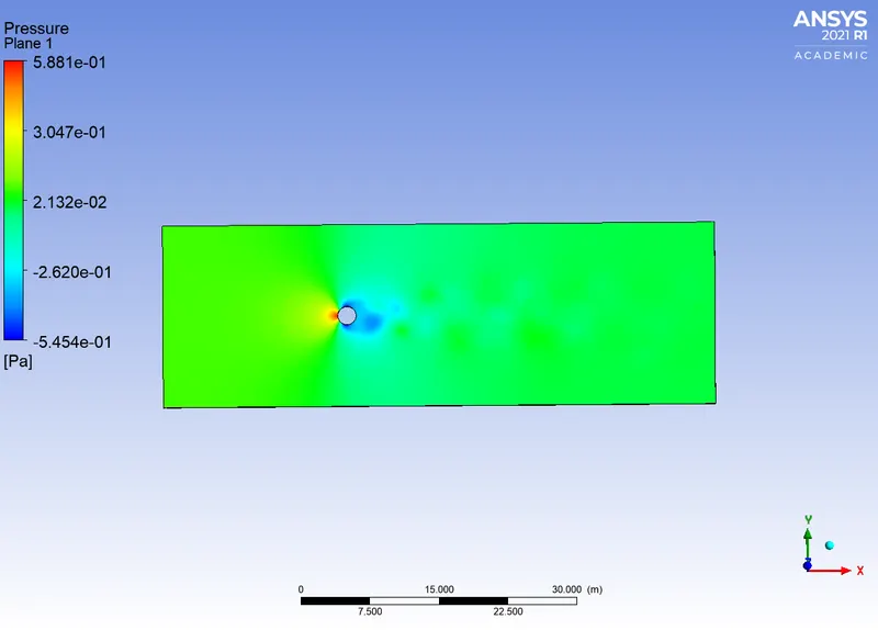
Transient state simulation at (Re = 100)

Scaled Residuals graph

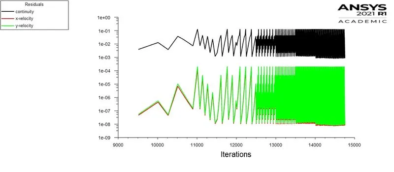
• From the above plot, it can be seen that the residuals variation do not hold the correct indication. It keeps changing every 5000 iterations.

Vertex average velocity at the monitor point

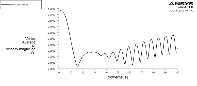
• The above monitor point velocity plot is obtained by observing the velocity at a monitor point created at a distance of 6m (3 times the diameter of the cylinder) axially.
• After about 100s, the oscillation is same. Hence, we can conclude that the solution has been converged at around 15000 to 16000 iterations.

Coefficient of lift

Strouhal Number

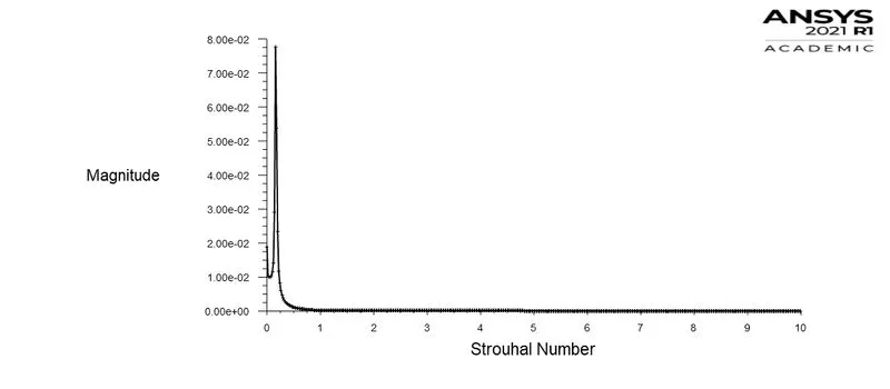
• From the above graph, we have found out the strouhal number (Sr) with case set-up 'Re =100' as 0.14435 corresponding to the highest magnitude value.

EXACT SOLUTION:

• Frequency of the vortex shedding 'f= no.of cycles / Time taken'

`f=4/(95-40)=0.07273`Hz

`Sr=(f.D)/v=(0.07273*2)/1=0.145`

• Therefore, the strouhal number calculated analytically matches with the computational value.

Velocity Contour

At CFD Post

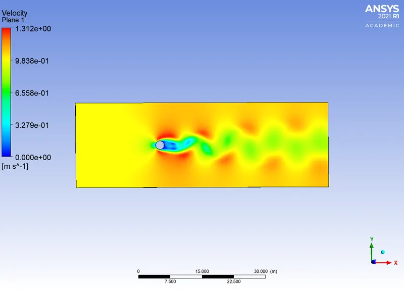
Pressure contour

At CFD Post

Vortex shedding Animation

• Animation Link : https://youtu.be/QEKgutb4woU

2) Calculation of coefficient of drag `(C_d)` and lift `(C_L)` over a cylinder by setting the Reynolds number to 10,100,1000,10000 & 100000. (Run with steady state solver)

Varying the Reynold's Number (Re):

• The values of diameter of the cylinder (D) and dynamic vsicosity of the fluid`(mu)` has to be kept constant while changing the velocity of the flow at the inlet to get the required Reynold's number value.
• For Example, `Re=(rhovD)/mu`

`Re= (1*1*2)/0.02=100`

Here, `D=2m`and `mu=0.02 (kg)/(m.s)`

So to get Re=100, the velocity value has to be 1m/s

• Similarly, the other required values of Reynold's number can be obtained by changing the velocity values accordingly.

`C_d` at Re=10,

`C_L` at Re=10,

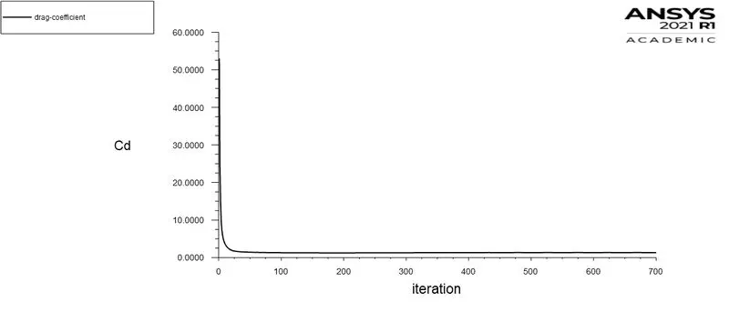
`C_d` at Re=100,

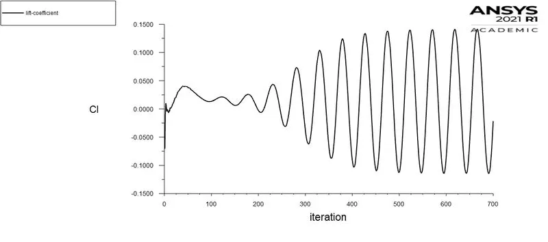
`C_L` at Re=100,

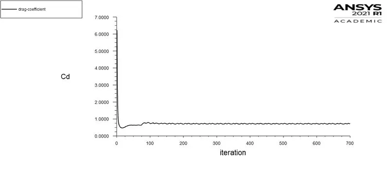
`C_d` at Re=1000,

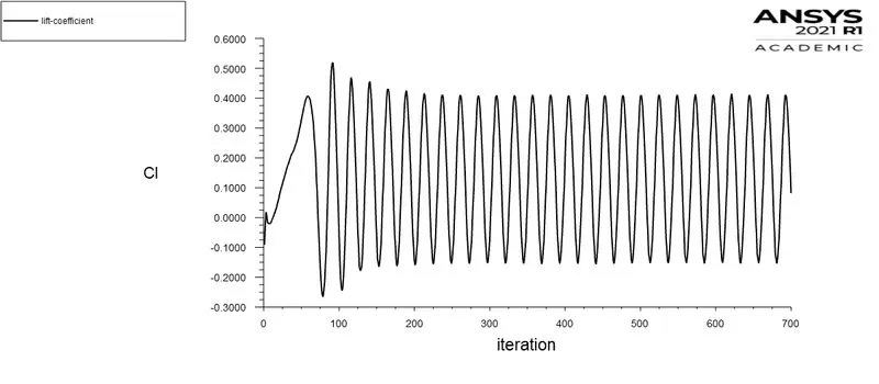
`C_L` at Re=1000,

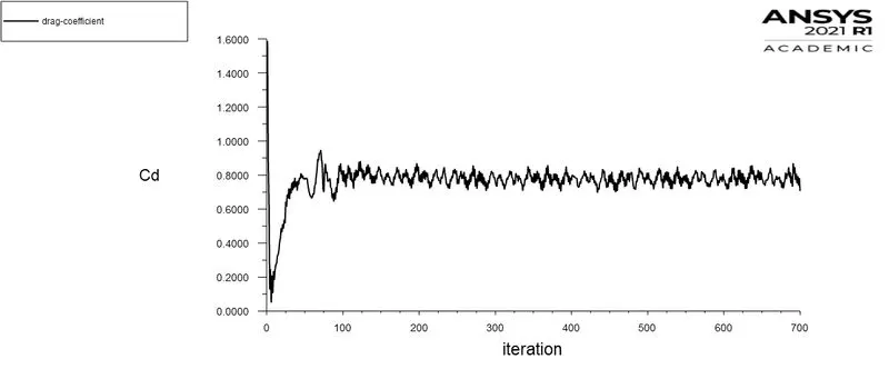
`C_d` at Re=10000,

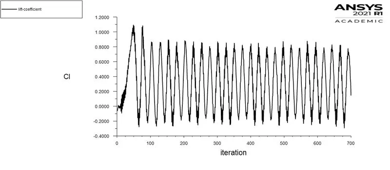
`C_L` at Re=10000,

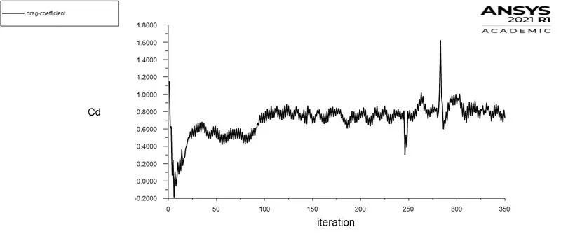
`C_d` at Re=100000,

`C_L` at Re=100000,

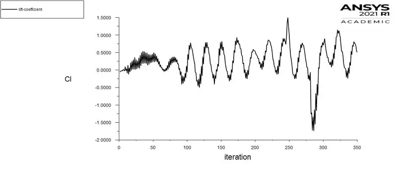
The values of `C_d` and `C_L` are tabulated below,

Velocity of flow `v`	Reynold's Number 'Re'	Coefficient of Drag `C_d`	Coefficient of Lift `C_L`
0.1	10	3.3252	0.00096
1	100	1.3348	-0.0215
10	1000	0.7170	0.0811
100	10000	0.7059	0.1437
1000	100000	0.7235	0.0548

CONCLUSION

• The simulation of flow over a cylinder to study the phenomenon of Von Karman vortex street has been done successfully using the ANSYS software.
• From Part 1, we can see that the Transient state simulation captures vortex shedding phenomenon more accurately than the Steady state simulation because of its no of time steps and time step size.
• The Karman vortex street has been visualized and variation of the velocity of flow studied at the wake after the cylinder.
• Also, the simulations have attained convergence for both steady state and transient state and this has been confirmed using the scaled residuals plot values.
• In Part 2, From the above table of `C_d` and `C_L` values at different Reynold's number , it is clear that the Reynold's number (Re) is inversely proportional to coefficient of drag which is as the Reynold's number increases ,the value of coefficient of drag decreases.
• It is obvious from the equations of Reynold's number and Coefficient of drag, where Reynold's number formula is directly proportional to the velocity of the flow and drag coefficient formula is inversely proportional to the velocity.
• The coefficient of drag value at `Re=100` is verified by referring to a research paper on "Numerical simulation of laminar flow past a circular cylinder (1)".
• In the journal, the value of `C_d` at `Re=100` for two-dimensional simulation is 1.3353.
• Whereas, On comparing this value with the calculated value of 1.3348, the absolute error is found out to be 0.05%. Hence, the simulation results are validated with the standard literature.

REFERENCE

1) N. Rajani , A. Kandasamy , Sekhar Majumdar , "Numerical simulation of laminar flow past a circular cylinder" , 2008.

https://www.sciencedirect.com/science/article/pii/S0307904X08000243