Week - 2 - Explicit and Implicit Analysis
Objective:
To solve Explicit and Implicit Methods using this given equation `f(u) = u^3+9u^2+4u`
Contrive the values with a residual tolerance of `10^2`
Explicit Method vs Implicit Method
Explicit analysis works in a way, that we don’t have to converge each step. There are no convergence criteria to check and no iterations. Time increment in the explicit analysis is very short i.e. impact wave
Implicit analysis works in a way, that in each time increment, the global equilibrium in the model is established. This means that each increment has to converge
Procedure:
Explicit analysis
Clearly, it is possible to plot a graph of force, f, versus displacement, u, by using an equation. However, if the nonlinear force versus displacement relationship is not known, but the stiffness is known, it is possible to construct the graph of force versus displacement numerically. One method is to use an incremental explicit load control scheme. This is illustrated next. For this example, three equal load increments (or steps) of `DeltaF = 1` unit each are used to load the tension bar. The variables used are u for displacement, f for internal force in the bar, F for the external force applied to the bar, and k for stiffness. Incremental displacements or incremental externally applied forces are represented as `DeltauorDeltaF`, respectively. Use is made of the relationship `DeltaF=kDeltau`. The analysis proceeds as follows: If the nonlinear force versus displacement relationship is not known, but the stiffness is known.
The following equation is solved using the explicit method as follows,
`f(u) = u^3+9u^2+4u`
A differentiating force with respect to displacement gives the stiffness(k) of the bar (since F = kx)
`k(u) = (df)/(du) = 3u^2+18u+4`
Here, three equal load increments (or steps) of `ΔF = 1`unit
The variables used are u for displacement, `f` for internal force in the bar, `F` for the external force applied to the bar, and `k` for stiffness. Incremental displacements or incremental externally applied forces are represented as `Δu or ΔF,` respectively.
`ΔF=k.Δu` This relation is used to find the incremental displacement
`bb "Step-1"`
Initial, `u_0=0; rArrk(u_0)=3(0)^2+18(0)+4rArr4; DeltaF= 1`
Changing, `Deltau_1=(DeltaF)/(K(u_0))rarr1/4rArr0.25`
Final, `u_1=Deltau_1+u_0rarr0.25+0rArr0.25`
`F_(Internal) = u^3+9u^2+4u rarr0.25^3+9(0.25)^2+4(0.25)rArr1.5781 ; F_(external)=DeltaFrArr1`
`R=F_(Internal)-F_(external)rarr1.5781-1rArr0.5781`
`bb "Step-2"`
Initial, `u_1=0.25; rArrk(u_1)=3(0.25)^2+18(0.25)+4rArr8.6875; DeltaF= 1`
Changing, `Deltau_2=(DeltaF)/(K(u_1))rarr1/8.6875rArr0.1151`
Final, `u_2=Deltau_2+u_1rarr0.1151+0.25rArr0.3651`
`F_(Internal) = u^3+9u^2+4u rarr0.3651^3+9(0.3651)^2+4(0.3651)rArr2.7086 ; F_(external)=DeltaF+DeltaFrArr2`
`R=F_(Internal)-F_(external)rarr2.7086-2rArr0.7086`
`bb "Step-3"`
Initial, `u_2=0.3651; rArrk(u_2)=3(0.3651)^2+18(0.3651)+4rArr10.9716; DeltaF= 1`
Changing, `Deltau_3=(DeltaF)/(K(u_2))rarr1/10.9716rArr0.0911`
Final, `u_3=Deltau_3+u_2rarr0.0911+0.3651rArr0.4562`
`F_(Internal) = u^3+9u^2+4u rarr0.4562^3+9(0.4562)^2+4(0.4562)rArr3.7927 ; F_(external)=DeltaF+DeltaF+DeltaFrArr3`
`R=F_(Internal)-F_(external)rarr3.7927-3rArr0.7927`
The external and internal forces are NOT in equilibrium `F_(External)≠F_(Internal)`
| `Step i` | `DeltaF_i` | `Deltau_i` | `u_i` | `(F_(External))_i` | `(F_(Internal))_i` | `R= F_(Internal)-F_(External)` |
| 1 | 1.0 | 0.25 | 0.25 | 1.0 | 1.5781 | 0.5781 |
| 2 | 1.0 | 0.1151 | 0.3651 | 2.0 | 2.7086 | 0.7086 |
| 3 | 1.0 | 0.0911 | 0.4562 | 3.0 | 3.7927 | 0.7927 |
Implicit analysis
An implicit analysis is the same as an explicit analysis, except that at the end of each step Newton-Raphson iterations are used to enforce equilibrium before moving to the next step. Basically, an incremental force is applied to advance the solution forward at the beginning of a step. However, internal forces and external forces will not be in equilibrium unless the stiffness is linear for the given step. Hence, in order to achieve equilibrium, corrections must be made to the displacement. This is accomplished by using Newton-Raphson iterations to minimize the residual, `R(u) = F_(Int) − F_(Ext)`.
Expanding the residual as a Taylor series about the current displacement `u^j` gives
`R^(j+1) = R^j(uj) + dR(u^j)/(du) deltau^(j+1) + ... = R^j + k(u^j)deltau^(j+1) + ...`
By neglecting higher order terms in the series, setting `R^(j+1) = 0` and solving for `deltau^(j+1)` the following correction is obtained
`deltau^(j+1) = −[k(u^j)]^(−1)R^j `
`bb "Step-1"`
Initial, `u_0=0; rArrk(u_0)=3(0)^2+18(0)+4rArr4; DeltaF= 1`
Changing, `Deltau_1=(DeltaF)/(K(u_0))rarr1/4rArr0.25`
Final, `u_1=Deltau_1+u_0rarr0.25+0rArr0.25`
`F_(Internal) = u^3+9u^2+4u rarr0.25^3+9(0.25)^2+4(0.25)rArr1.5781 ; F_(external)=DeltaFrArr1`
`R=F_(Internal)-F_(external)rarr1.5781-1rArr0.5781`
`R > 10^(−2) rArr` Newton-Raphson iterations are necessary
Second iterations,
`u_1 = u_1^((0)) rArr 0.25`
`deltau^(1) = −[k(u_1^0)]^(−1)R^0 rarr -(0.5781)/(8.6875) rArr 0.0655`
`u_(1)^((1))=deltau^1+u_(1)^((0))rarr-0.665+0.25rArr0.1835`
`F_(Int)=u^3+9u^2+4u rarr 0.0062+0.3030+0.734 rArr 1.4032`
`F_(ext)=DeltaFrArr1`
`R^(0)=F_(Int) - F_(Ext) rarr 1.0432-1 rArr .0432`
`R^(0) > 10^(−2) rArr` Newton-Raphson iterations are necessary
Third iterations,
`u_1 = u_1^((1)) rArr 0.1835; deltau_(1)=-0.0665; R_(0)=0.432`
`deltau^(2)=deltau_(1)−[k(u_1^1)]^(−1)R^0 rarr -0.0665-(0.0432)/(7.4040) rArr -0.723`
`u_(1)^((2))=deltau_(1)^((2)) + u_(1)^((0))rarr-0.0723+0.25rArr0.1777`
`F_(Int)=u^3+9u^2+4u rarr 0.0056+0.2842+0.7108 rArr 1.0005`
`F_(ext)=DeltaFrArr1`
`R^(1)=F_(Int) - F_(Ext) rarr 1.0005-1 rArr .0005`
`R^(1) 10^(−2)` No iterations are necessary
`bb "Step-2"`
Initial, `u_1=0.1777; rArrk(u_1)=3(0.1777)^2+18(0.1777)+4rArr7.2933; DeltaF= 2`
Changing, `Deltau_2=(DeltaF)/(K(u_1))rarr1/7.2933rArr0.1371`
Final, `u_2=Deltau_2+u_1rarr0.1371+0.1777rArr0.3148`
`F_(Internal) = u^3+9u^2+4u rarr0.3148^3+9(0.3148)^2+4(0.3148)rArr2.1821 ; F_(external)=DeltaFrArr2`
`R=F_(Internal)-F_(external)rarr2.1821-2rArr0.1821`
`R > 10^(−2) rArr` Newton-Raphson iterations are necessary
Second iterations,
`u_2= u_2^((0)) rArr 0.3148`
`deltau^(1) = −[k(u_2^0)]^(−1)R^0 rarr -(0.1821)/(9.9636) rArr -0.0182`
`u_(2)^((1))=deltau^1+u_(2)^((0))rarr-0.0182+0.3148rArr0.2965`
`F_(Int)=u^3+9u^2+4u rarr 0.026+0.791+1.186 rArr 2.003`
`F_(ext)=DeltaFrArr2`
`R^(1)=F_(Int) - F_(Ext) rarr 2.003-2 rArr .003`
`R^(1) < 10^(−2)`no iterations are necessary
`bb "Step-3"`
Initial, `u_2=0.2965; rArrk(u_2)=3(0.2965)^2+18(0.2965)+4rArr0.1041; DeltaF= 3`
Changing, `Deltau_3=(DeltaF)/(K(u_2))rarr1/9.6007rArr0.1041`
Final, `u_3=Deltau_3+u_2rarr0.1041+0.2965rArr0.4006`
`F_(Internal) = u^3+9u^2+4u rarr0.4006^3+9(0.4006)^2+4(0.4006)rArr3.1109 ; F_(external)=DeltaFrArr3`
`R=F_(Internal)-F_(external)rarr3.1109-3rArr0.1109`
`R > 10^(−2) rArr` Newton-Raphson iterations are necessary
Second iterations,
`u_3= u_3^((0)) rArr 0.4006`
`deltau^(1) = −[k(u_3^0)]^(−1)R^0 rarr -(0.1109)/(11.6922) rArr -0.0094`
`u_(3)^((1))=deltau^1+u_(3)^((0))rarr-0.0094+0.4006rArr0.3912`
`F_(Int)=u^3+9u^2+4u rarr 0.0598+1.3773+1.5648 rArr 3.0019`
`F_(ext)=DeltaFrArr3`
`R^(1)=F_(Int) - F_(Ext) rarr 3.0019-3 rArr .0019`
`R^(1) < 10^(−2)`no iterations are necessary
| `Step i` | `DeltaF_i` | `u_i` | `(F_(External))_i` | `(F_(Internal))_i` | `R= F_(Internal)-F_(External)` |
| 1 | 1.0 | 0.1777 | 1.0 | 1.0005 | 0.0005 |
| 2 | 1.0 | 0.2965 | 2.0 | 2.0030 | 0.0030 |
| 3 | 1.0 | 0.3912 | 3.0 | 3.0019 | 0.0019 |
`bb "Step-1"`
External energy values are solved in the quadratic equation `ax^3+bx^2+cx+d` to obtain the values of `U_(exact)` with `a =1 , b = 9, c = 4 and d =deltaF`
`ax^3+bx^2+cx+d` `rarr` `1x^3+9x^2+4x=-1` `rArr` `x_(1) = 0.17762 ;x_(2) = -8.51654; x_(3) = -0.66108`
We should claim the positive value as `U_(exact) = 0.177`
Similarly by following the above method for `"Steps 2&3"` respectively to derive the values `u_(2)=0.2966 ; u_(3)= 0.3911`
| `Step i` | `Force` | `Explicit` | `Implicit` | `U_(Exact)` |
| 1 | 1.0 | 0.25 | 0.1777 | 0.1776 |
| 2 | 2.0 | 0.3651 | 0.2965 | 0.2966 |
| 3 | 3.0 | 0.4562 | 0.3912 | 0.3911 |
Graph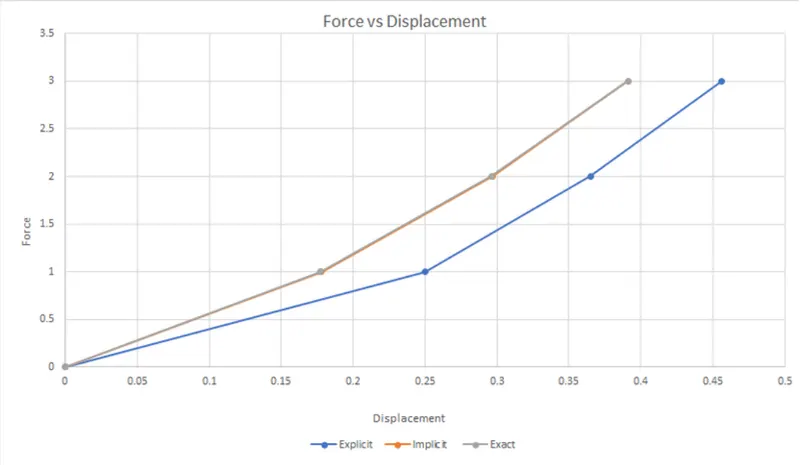
- From the above graph, it is clear that the Explicit analysis drift away from the exact solution this illustrates the lack of equilibrium between internal and external energies
- Whereas in the case of Implicit analysis the lack of equilibrium is cleared by using Newton-Raphson Iteration to correct the incremental step so that the analysis will give exact result as observed in the graph
Conclusion
A Non-linear analysis is tabulated and plotted the graphical representation by using the incremental explicit and implicit procedure using this given equation `f(u) = u^3+9u^2+4u` with a residual tolerance of `10^2`