Week - 2 - Explicit and Implicit Analysis
Introduction:
When a Structure response ( deformation, stress and strain ) is linearly proportional to the magnitude of the load ( Force, Pressure, moment, torque, temp etc.,) then the analysis of a structure is known as linear analysis whereas the load to response relationship is not linearly proprortional then the analysis is called Non linear analysis most of the real time analysis will be non linear in nature . The stiffness matrix relating to the load and response is assumed to be constant in the case of static analysis however it is not possible in realtime the non linear analysis will consider geometrical factors such as length, cross section, area and moment of inertia etc., as well as material properties such as elastic modulus, rigidity modulus etc., These changes are accomodated into the analysis by rebuilding the stiffness matrix using deformed structure configuration and updated property after each incremental load application. there are two approaches in FE for these non linaear analysis namely Implicit and Explicit analysis.
Explicit Analysis:
An Explicit analysis does the incremental procedure and at the end of each increment updates the stiffness matrix based on geometry changes and material changes. Then a new stiffness matrix is constructed and the next increment of load (or displacement) is applied to the system. In this type of analysis the hope is that if the increments are small enough the results will be accurate. One problem with this method is that you do need many small increments for good accuracy and it is time consuming. most importantly, this method does not enforce equilibrium of the internal structure forces with the externally applied loads.The explicit analysis offers a faster solution in the events where there is a dynamic equilibrium (i.e) Sum of all forces = mass x acceleration, These events can be best exampled by extreme scenarios such as an automotive crash, ballistic event, or even meteor impact. In these cases, the material models do not only need to account for the variation of stress with strain but also the strain rate. On this scale, the strain rates play a particularly important contribution.
Applications: For wave propagation types of problems such as crash analysis, drop, blast, etc.
Impicit Analysis:
An Implicit analysis is the same as Explicit with the addition that after each increment the analysis does Newton-Raphson iterations to enforce equilibrium of the internal structure forces with the externally applied loads. The equilibirium is usually enforced to some user specified tolerance.So this is the primary difference between the two types of anlysis, This type of analysis tends to be more accurate, One draw back of the method is that during the Newton-Raphson iterations one must update and reconstruct the stiffness matrix for each iteration.This can be computationally costly, If done correctly the Newton-Raphson iterations will have a quadratic rate of convergence which is very desireable. An implicit analysis finds a solution by solving an equation that includes both current and later states of the system, Impicit method is used in softwares suchs as ansys, nastran, abaqus etc.,
Procedure:
Simplification using Explicit analysis:
The Given Equation F(u) = u³+9u²+4u is calculated by explicit method........................(eqn 1)
Ans: The stiffness equation is defined by K = df/du
By differentiating with respect to u we get k(u) = df/du = `3u^2+18u+4'.....................(eqn 2)
The relation `delF=kdelu`can be used to find incremental displacement
where,
F = External force
u = displacement
`delF`= Incremental force
`del U`= Incremental displacement
Step 1
now to get U_0
K(`u_0`) = `3(0)^2+18(0)+4` ................................. ( from eqn 2)
K(`u_0`) = 4
We know that `del U_1= (delF)/(K(u_0)`
= 1/4
`del U_1` = 0.25
`implies` `U_1` = `del U_1` + 0 = 0.25
Substitute `U_1`in Force function `F(U_1)`.................. ( from eqn 1)
`F(U_1)` = `0.25^3+ 9(0.25)^2+4(0.25)`
`F(U_1)` = 1.578
Residual `R^0 =` (F_(Internal))_1-(F_(
`implies` `R^0 = 0.5781
U_(exact) = 0.177
Step 2
now to get U_1
K(`u_1`) = `3(0.25)^2+18(0.25)+4` ................................. ( from eqn 2)
K(`u_1`) = 8.6875
We know that `del U_2= (delF)/(K(u_1)`
= 1/8.6875
`del U_2` = 0.1151
`implies` `U_2` = `del U_2` + `U_1`
= 0.1151 + 0.25
`U_2` = 0.3651
Substitute `U_2`in Force function `F(U_2)`.........................( From eqn 1)
`F(U_2)` = `0.3651^3+ 9(0.3651)^2+4(0.3651)`
`F(U_2)` = 2.708
Residual `R^0 =` (F_(Internal))_2 - (F_(
`implies` `R^0 = 0.708
U_(exact) = 0.296
Step 3
now to get U_2
K(`u_2`) = `3(0.3651)^2+18(0.3651)+4` ................................. ( from eqn 2)
K(`u_2`) = 10.9716
We know that `del U_3= (delF)/(K(u_2)`
= 1/10.9716
`del U_3` = 0.0911
`implies` `U_3` = `del U_3` + `U_2`
= 0.0911 + 0.3651
`U_3` = 0.4562
Substitute `U_3`in Force function `F(U_3)`.........................( From eqn 1)
`F(U_3)` = `0.4562^3+ 9(0.4562)^2+4(0.4562)`
`F(U_3)` = 3.7928
Residual `R^0 =` (F_(Internal))_3 - (F_(
`implies` `R^0 = 0.7928
U_(exact) = 0.391
External energy values are solved in the quadratic equation ax^3+bx^2+cx+d` to obtain the values of U_(exact) with a =1 , b = 9, c = 4 and d = `del F`
Table 1: Summary of explicit analysis
| `Step_i` | `del F_i` | `del u_i` | `u_i` | (F(ext))_i | (F(int))_i | Residual `R^0` | U_exact |
| 1 | 1 | 0.25 | 0.25 | 1 | 1.578 | 0.578 | 0.177 |
| 2 | 1 | 0.1151 | 0.3651 | 2 | 2.708 | 0.708 | 0.296 |
| 3 | 1 | 0.0911 | 0.4562 | 3 | 3.972 | 0.972 | 0.391 |
from the table it can be seen that the internal energy is not in equilibrium with the external energy
Simplification using Implicit analysis:
Implicit analysis is same as that of explicit analysis except that at the end of each step equilibrium is achieved through Newton-Raphson Iteration, basically an incremental force is applied to advance the solution forward at the begining of a step however the internal and external forces will not be in equilibrium unless the stiffness is linear for the given step hence to achieve equilibrium correction must be made to the displacement.
The Given Equation F(u) = u³+9u²+4u is calculated by implicit method........................(eqn 1)
Iteration variable is j and it may take several iterations for the norm of the residual, `||R||`, to be reduced below the chosen tolerance criteria (for the example below a tolerance of `10^-2`is chosen)
The stiffness equation is defined by K = df/du
By differentiating with respect to u we get k(u) = df/du = `3u^2+18u+4'.....................(eqn 2)
The relation `delF=kdelu`can be used to find incremental displacement
Step 1
now to get U_0
K(`u_0`) = `3(0)^2+18(0)+4` ................................. ( from eqn 2)
K(`u_0`) = 4
We know that `del U_1= (delF)/(K(u_0)`
= 1/4
`del U_1` = 0.25
`implies` `U_1` = `del U_1` + 0 = 0.25
Substitute `U_1`in Force function `F(U_1)`.................. ( from eqn 1)
`F(U_1)` = `0.25^3+ 9(0.25)^2+4(0.25)`
`F(U_1)` = 1.578
Residual `R^0 =` (F_(Internal))_1-(F_(
`implies` Residual `R^0 = 0.5781
Here the Residual (`R^0`) = 0.578 is greater that `10^-2` so the Newton-Raphson iterations are applied to the function
Iteration 1 :
Let us consider `u_1= u_(1)^0`
`del u^1 = - [K(u_(1)^0)]^-1*R^0`
(u_(1)^0) = `3u^2+18u+4`
`implies` Ku_(1)^0` = `3(0.25)^2+18(0.25)+4`....................( Sub (u_(1)^0) = 0.25 )
Ku_(1)^0` = 8.6875
`del u^1` = 0.5678/0.86675
`del u^1` = 0.666
`u_1^1` = `del u^1`+ `u^0` = 0.666+0.25
`u_1^1` = 0.184
Substitute `u_1^1`in Force function `F(`u_1^1`)`.................. ( from eqn 1)
`F(`u_1^1`)` = `0.184^3+ 9(0.184)^2+4(0.184)`
`F(`u_1^1`)` = 1.0469
Residual `R^1 =` (F_(Internal))_1-(F_(
`implies``R^1 = 0.0469
Here the Residual (`R^1`) = 0.0469 is greater that `10^-2` so another iterations is applied to the function
Iteration 2:
Let us consider `u_1= u_(1)^1`
`del u^2` = - [K(u_(1)^1)]^-1*R^1`
(u_(1)^1) = `3u^2+18u+4`
`implies` Ku_(1)^1` = `3(0.184)^2+18(0.184)+4`....................( Sub (u_(1)^1) = 0.184 )
Ku_(1)^1` = 7.413
`del u^2` = - 0.666*0.0469/0.86675
`del u^2` = -0.0723
`u_1^2` = `del u^2`+ `u^0` = - 0.723 +0.25
`u_1^2` = 0.178
Substitute `u_1^2`in Force function `F(`u_1^2`)`.................. ( from eqn 1)
`F(`u_1^2`)` = `0.178^3+ 9(0.178)^2+4(0.178)`
`F(`u_1^2`)` = 1.0027
Residual `R^2 =` (F_(Internal))_1-(F_(
`implies``R^2 = 0.002`
Here the Residual (`R^2`) = 0.0027 is less that `10^-2` so iterations can be stopped here
Similarly by following the above method for steps 2&3 respectively to derive the values `u_2 = 0.2966 & u_3` = 0.3911
Table 2: Summary of Implicit analysis
| `Step_i` | `del F_i` | `del u_i` | (F(ext))_i | (F(int))_i | Residual `R^0` | U_exact |
| 1 | 1 | 0.178 | 1 | 1.002 | 0.002 | 0.177 |
| 2 | 1 | 0.297 | 2 | 2.007 | 0.007 | 0.296 |
| 3 | 1 |
0.391 |
3 | 2.993 | 0.002 | 0.391 |
From the table it can be seen that the external and internal forces are converged before skipping from one cycle to another
Although the Internal and external energy Are not in equilibrium in Both Methos, Implicit has fewer errors compared with explicit this is because The analysis moves to the next step only when the convergence is achieved in the first step, thus the errors are small.
The results of explicit and Implicit are summarized in the table below.
Table 3:
| `Step_i` | Force | Implicit | Explicit | Exact |
| 1 | 1 | 0.178 | 0.25 | 0.177 |
| 2 | 2 | 0.297 | 0.3651 | 0.296 |
| 3 | 3 | 0.391 | 0.4562 | 0.391 |
GRAPH:
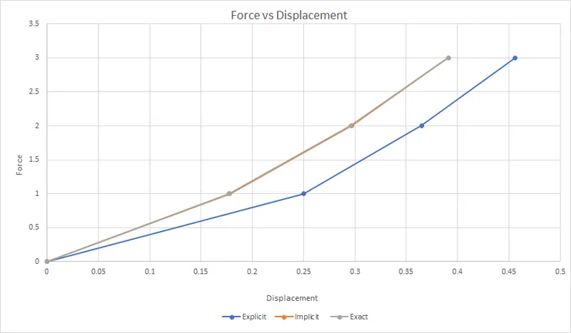
- From the above graph it is clear that the Explicit analysis drift away from the exact solution this illustrates the lack of lack of equilibrium between internal and external energies
- where as inthe case of implicit analysis the lack of equilibrium is cleared by using Newton-Raphson Iteration to correct the incremental step so that the analysis will give exact result as seen in the graph
Conclusion:
A Non linear analysis is done by using incremental explicit and implicit procedure and the results are tabulated and plotted in a graph from which it is evident that explicit analysis drifts away from the exact solution due to lack of equilibrium between internal and external forces which is overcomed by Newton-Raphson Iteration to enforce equilibrium in Implicit analysis,Newton Raphson Iterations are used for Convergence So that they can Replicate the exact solution According to the Given tolerance and the solution is achieved by the Iterations