Week - 2 - Explicit and Implicit Analysis

Aim:-

1. Write a detailed report about Implicit and explicit methods.
2. Solve the given partial differential equation uding both implicit and explicit scheme and plot the graphs for the same.

Introduction:-

Ls-Dyna is an advanced general purpose multophysies simulation software developed by the  Forme Liver more software Technology corporation, in 2019 it acquired by Ansys. Ls-Dyna is a solveer that solve linear or nonlinear problem of finite element analysis using implicit or explicit method.

Ls-Dyna is used by civil-engineering, autmobile, construction, manufacturing, aerospace and bioengineering industries.

Explicit and implicit schem 

• Explicit and implicit method's are approaches used in numerical analysis for obtaining numerical approximations to the solutions of time dependent ordinary and partial differential equations as is required in computer simulations of physical processes.
• Explicit and implicit problems are expressed mathematical partial sifferential equation. In current , we used computer to solve any problems they can't single-handedly solve partial differential equations instade of they are solve matrix equations. These equations can be linear or non-linear, in steuctural problems the non-linear equations devide into three categories.
• Material nonlinearity:- Where deformations and strains are large ex:- polymer materials like plastic, polyvinyl chloride etc
• Geometric nonlinearity:- Where strains are small but rotations are large ex:-thin structures
• Boundary nonlinearity:- Due to nonlinearity of boundary conditions ex:- contact problems

linear problems in a matrix equations

[k] {x}={ƒ}

nonlinear static problems

[k(x)] {x}={ƒ}

for dynamic problem the matrix equation

[M] {x"}+[C] {x'}+[K]{x}={ƒ}

physically these mean's

inertial force+damping force+stiffness force= external force

where

x"=accleration

x'=velocity

m=mass

c=damping

k=stiffness

f=external force

• Implicit analysis:- In this analysis we find the unknowns value through matrix inversion. It can be exteremely time-consuming when solving dynamic and nonlinear problems. This method also known as backward eular's integration becaus the solution for the current step is based on the previous step.
•  

             

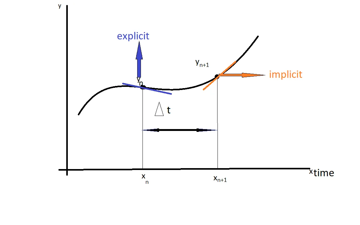
yn+1 =yn + Δtƒ{xn+1,yn+1}

where,

yn+1 is a unknown   ,   yn is a known, ƒ{xn+1,yn+1} is a unknown

• it unconditionally stable
• time step large

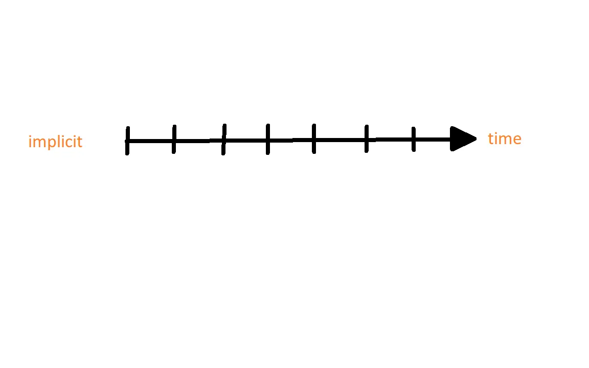
• for nonlinear problem need iterations
• solving speed for one step slow 
• use for creep,quasi-static, static/dynamic drop test
• Ecplicit analysis:- A scheme is explicit when the information at time level "n+1" depends on previous time level's "n,n-1" etc so it also known as eular integration
•        

yn+1 =yn + Δtƒ{xn,yn}

where,

yn+1 is a unknown   ,   yn is a known, ƒ{xn,yn} is a known

• time size requirement that smaller

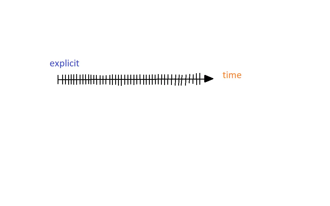
• stablity depends on time step size
• for nonlinear does't need iterations
• solving speed for one step fast
• use for drop test, impact

The problem:-As demonstrated in the PDF, F(u) = u3+9u2+4u use this equation and solve using both Explicit and Implicit Methods ( have a tolerence of 0.01).

consider the case of a simple bar in tension suppose that the force in the bar is a nonlinear function of the displacement 

ƒ(u)=u⊃;;3;+9u⊃;;2;+4u.....................(1)

from (1) it follows that the stiffiness of the bar is

k(u)=3u⊃;;2;+18u+4.........................(2)

Explicit calculation:-

three equal load increments of ΔF=1 unit each are used to load the tension bar.

the variable use are

u=displacement

ƒ=internal force in bar

F=external force applied on bar

k=stiffness

Δu=incremental displacements

ΔF=incremental externally applied forces

 use is made of the relationshipΔF=kΔu

Step1:-

form equation (2) put (uo)=0.0, then

k(uo)=3(uo)⊃;;2;+18(uo)+4=4

Δ(u1)=ΔF/k(uo)=1/4=0.25

now,

(u1)=(uo)+Δ(u1)=0.0+0.25=0.25

Step2:-

put (u1)=0.25 in eq (2)

k(u1)=3(u1)⊃;;2;+18(u1)+4=3(0.25)⊃;;2;+18(0.25)+4=8.69

ΔF=1

now,

Δ(u2)=ΔF/k(u1)=1/8.69=0.115

(u2)=(u1)+Δ(u2)=0.25+0.115=0.365

Step3:-

again eq (2) put (u2)=0.37

k(u2)=3(u2)⊃;;2;+18(u2)+4=3(0.37)⊃;;2;+18(0.37)+4=11.07

ΔF=1

now,

Δ(u3)=ΔF/k(u2)=1/11.07=0.0911

(u3)=(u2)+Δ(u3)=0.365+0.0911=0.456

Finally from the three steps the following results are obtaoned

F(ext)=ΔF+ΔF+ΔF=1+1+1=3

F(int)1=(u1)⊃;;3;+9(u1)⊃;;2;+4(u1)=(0.25)⊃;;3;+9(0.25)⊃;;2;+4(0.25)=1.578

F(int)2=(u2)⊃;;3;+9(u2)⊃;;2;+4(u2)=(0.365)⊃;;3;+9(0.365)⊃;;2;+4(0.365)=2.708

F(int)3=(u3)⊃;3;+9(u3)⊃;2;+4(u3)=(0.456)⊃;3;+9(0.456)⊃2;+4(0.456)=3.7908

it is evident from the results that external and internal force are not in equilibrium because

F(ext)≠F(int)

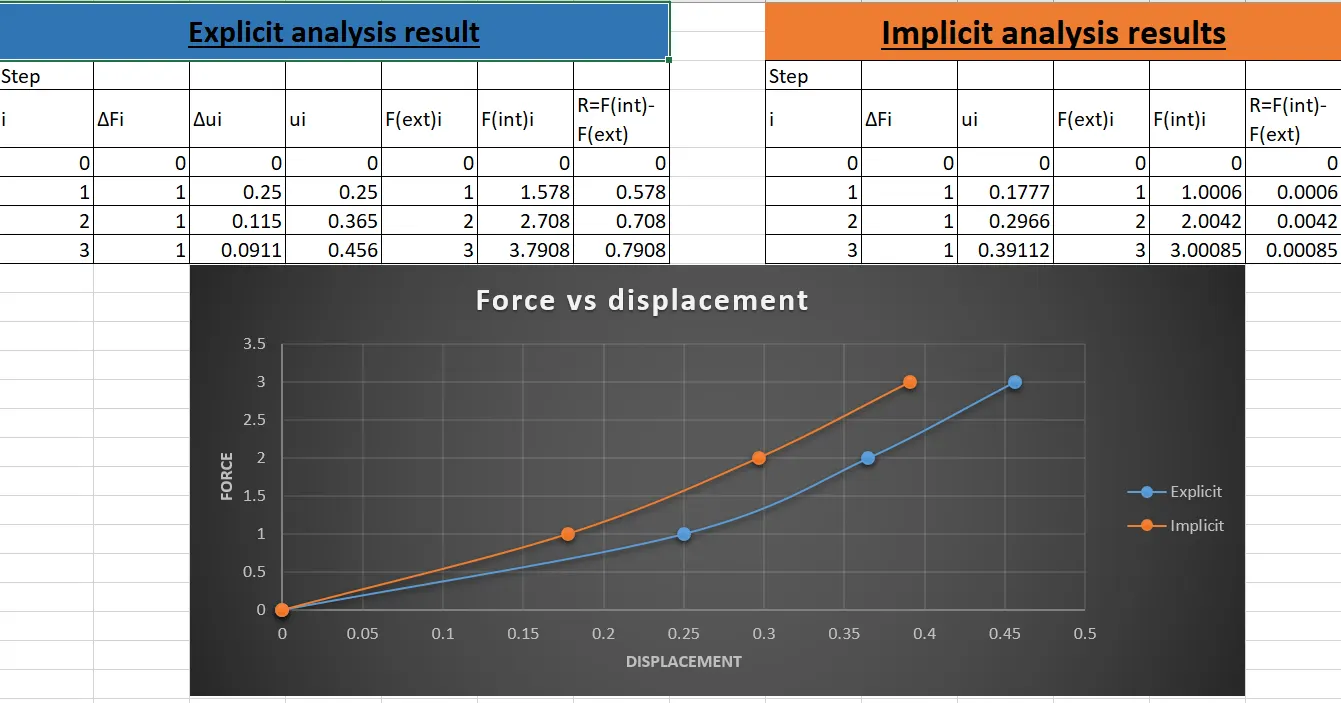
Explicit analysis result:-

Step
i	ΔFi	Δui	ui	F(ext)i	F(int)i	R=F(int)-F(ext)
1	1	o.25	0.25	1.0	1.578	0.578
2	1	0.115	0.365	2.0	2.708	0.708
3	1	0.0911	0.456	3.0	3.7908	0.7908

Implicit calculation:-

Implicit analysis is the same as the explicit analysis except that at the end of each step newton-raphson iteration are used to enforce equilibrium before moving to the next step. Basically an incremental force is applied to advance the solution forward at the beginning if a step, However internal forces and external force will not be in equilibrium unless the stiffness is linear for the given step, Hence to achive equilibrium corrections must be mase to the displacement.this is accomplished by using newton-raphson iterations to minimize the residual 

R(u)=F(int)-F(ext)

expanding the residual as a Taylor series about the  current displacement u^j gives

R^(j+1)=R^j(u^J)+dR(u)^j/du*δu^j+1....

            =R^j+k(u^J)δu^j+1...........

By neglecting higher order terms in the series setting R^j+1 and solving for δu^j+1 the following correction is obtained

δu^j+1=-[k(u^j)]^-1*R^j

j=iteration variable

Step1:-

uo=0.0 then

k(uo)=3(uo)^2+18(uo)+4=4

ΔF=1

ΔF=Δu1*k(uo)

Δu1=ΔF/k(uo)=1/4=0.25

u1=uo+Δu1=0.0+0.25=0.25

chack the residual

F(ext)=ΔF=1

F(int)=u1^3+9u1^2+4u1=(0.25)^3+9(0.25)^2+4(0.25)=1.578

R(o)=F(int)-F(ext)=1.578-1=0.578

R(o)>10^-2

Newton-Raphson iterations are necessary

calculate the correction to

u1=uo=0.25

k(uo)=3(uo)^2+18(uo)+4=3(0.25)^2+18(0.25)+4=8.6875

then,

δu1=-1/k(uo)*R(o)=-1/8.6875*0.578=-0.0665

the updared value of

u1^(1)=u1^(o)+δu1=0.25+(-0.0665)=0.1835

chack the residual again

F(ext)=1

F(int)=(u1^(1))^3+9(u1^(1))^2+4(u1^(1))=(0.1835)^3+9(0.1835)^2+4(0.1835)=1.0432

R(1)=F(int)-F(ext)=1.0432-1=0.0432

R(1)>10^-2

so another Newton-Raphson iteration is necessary

calculate the new to correction u1^(1)=uo

k(u1(1))=3(u1^(1))^2+18(u1^(1))+4=3(0.1835)^2+18(0.1835)+4=7.4040

δu2=δu1-1/k(u1(1))*R(1)=-0.0665-1/7.4040*0.0432=-0.07233

the updated value of

u1^(2)=u1^(0)+δu2=0.25+(-0.0732)=0.1777

chack the residual

F(ext)=1

F(int)=(u1^(2))^3+9(u1^(2))^2+4(u1^(2))=(0.1777)^3+9(0.1777)^2+4(0.1777)=1.0006

R(2)=F(int)-F(ext)=1.0006-1=0.0006

R(2)<10>

no further iterations are necessary 

Therefore the funal value is u1=u1^(2)=0.1777

Step2:-

k(u1)=3(u1)+18(u1)+4=3(0.1777)^2+18(0.1777)+4=7.293

ΔF=1

Δu2=ΔF/k(u1)=1/7.293=0.1371

u2=u1+Δu2=0.1777+0.1371=0.3148

chack the residual

F(ext)=ΔF+ΔF=2

F(int)=(u2)^3+9(u2)^2+4(u)=(0.3148)^3+9(0.3148)^2+4(0.3148)=2.1822

R(o)=F(int)-F(ext)=2-2.1822=0.1822

R(o)>10^-2

Newton-Raphson iterations are necessary

calculate the correction to 

u2=u2^(o)=0.3148

k(u2^(o))=3(u2^o)^2+18(u2^o)+4=3(0.3148)^2+18(0.3148)+4=9.963

δu1=-1/k(u2^o)*R(o)=-1/9.963*0.1822=-0.0183

update value of u2^1=u2^o+δu1=0.3148+(-0.0183)=0.2966

chack the residual again

F(ect)=2

F(int)=(u2^1)^3+9(u2^1)^2+4(u2^1)=(0.2966)^3+9(0.2966)^2+4(0.2966)=2.0042

R(1)=F(int)-F(ext)=2.0042-2=0.0042

R(1)<10>

Newton-Raphson iterations are no necessary

Therefor the final value is u2=u2^1=0.2966

Step3:-

u2=0.2966 then,

k(u2)=3(u2)^2+18(u2)+4=3(0.2966)^2+18(0.2966)+4=9.6027

ΔF=1, thenΔu3=ΔF/k(u2)=1/9.6027=0.1041

u3=u2+Δu3=0.2966+0.1041=0.4007

chack the residual

F(ext)=3

F(int)=(u3)^3+9(u3)^2+4(u3)=(0.4007)^3+9(0.4007)^2+4(0.4007)=3.1121

R(o)=F(int)-F(ext)=3.1121-3=0.1121

R(o)>10^-2

Newton-Raphson iterations are necessary

calculate thecorrection to u3=u3^o=0.4007

k(u3^o)=3(u3^O)^2+18(u3^o)+4= 3(0.4007)^2+18(0.4007)+4=11.6943

δu1=-1/k(u3^o)*R(o)=-1/11.6943*R(1)=-1/11.6943*0.1121=-0.009585

updated value u3^1=u3^o+δu1=0.4007-0.00958=0.39112

chack the residual again 

F(ext)=3

F(int)=(u3^1)^3+9(U3^1)^2+4(u3^1)=(0.39112)^3+9(0.39112)^2+4(0.39112)=3.00085

R(1)=F(int)-F(ext)=3.00085-3=0.00085

R(1)<10>

Newton-Raphson iterations are not necessary

Therefore the final value is u3=u3^1=0.39112

Implicit analysis results:-

Step
i	ΔFi	ui	F(ext)i	F(int)i	R=F(int)-F(ext)
1	1	0.1777	1	1.0006	0.0006
2	1	0.2966	2	2.0042	0.0042
3	1	0.39112	3	3.00085	0.00085

Conclusion:-

• The aim of the week2 challenge were to write a detailed repotr about implicit and explicit methods and also solve the given partial differentian equation using implicit and explicit methods.
• the result obtained using both schemes were plotted to understand which of the schemes yield better and effective result.
• the result presented that the explicit analysis drifts from the true solution illustrating the lack of equilibrium between the internal and external forces. 
• To overcome this problem an implicit analysis should be used,which include Newton-Rapohson iterations to enforce equilibrium betweeen internal and external forces.