Week - 2 - Explicit and Implicit Analysis

EXPLICIT AND IMPILICIT ANALYSIS

AIM:

To solve the non linear static problem of displacement equation F(u) = u³ + 9u²+4u is using explicit method and implicit method with a tolerance of 0.001.

OBJECTIVE :

• To provide an explanation about explicit and implicit method of analysis.
• To do numerical calculation of the explicit and implicit method of analysis.
• To plot the graph of explicit and implicit calculated values and compare the results.

DATA BASE :

1. Non linear static problem of displacement equation F(u) = u³ + 9u²+4u.
2. Tolerance value = 0.001.

(1)EXPLANATION ABOUT EXPLICIT AND IMPLICIT METHOD OF ANALYSIS.

EXPLICIT AND IMPLICIT TIME INTEGRATION

There are two ways in which dicretization process can be carried out,

1. Spatial or space discretization -is where the model with infinite DOF is converted into model with finite elements and DOFs.
2. Time discretization- is in which method one has to solve the physical problem that is provided, this is where explicit time integration and implicit time integration comes into play.

• Solving any physical problem is input quantity or filed variables = output quanity or filed variables.
• Since no body / system can have 100% efficiency, the above statement change as ,

Input quantity or filed variables = output quanity or filed variables + errors.

1. Explicit method

• Time dependant problems with Considering the velocity, acceleration , change in mass and inertia.
• Examples- car crash , tensile torsion test and phone drop test, ballistic events,blast events and metal stamping.
• No iterations.
• Conditionally stable , Courant-Fredrich-Levy(CFL) criteria
• Needs low memory
• Relatively smaller time steps
• Spatial derivative evaluated at 'n ' time in interval.
• Equation at time t , {F_n} = [M_n] {u^.._n} + [C_n] {u^._n} + [K_n] {u_n}
  

2.Implicit method

• In linear static analysis only force did not depend on time and dynamic loading occurs .
• Examples-applying load on a cantilever beam and buckling analysis, self weight, constant pressure loading,static forces and slowly applied displacement.
• Itertaions required for non linear probelm.
• Needs high memory.
• Large time steps and may change due to non linearities.
• Spatial derivative evaluated at 'n+1 ' time in interval.
• Equation at time t , {F_n+1} = [M_n+1] {u^.._n+1} + [C_n+1] {u^._n+1} + [K_n+1] {u_n+1}.

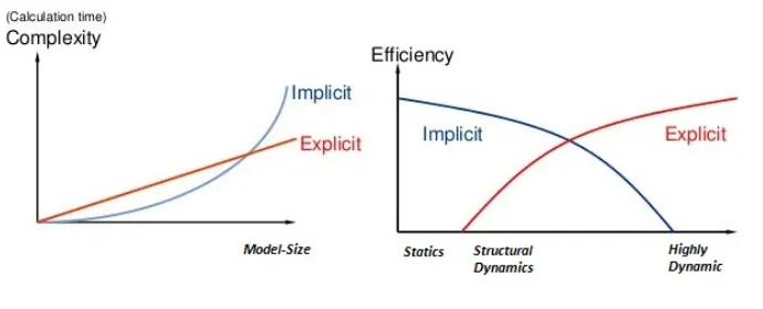
DIFFERENCE BETWEEN THE IMPLICIT AND EXPLICIT METHODS.

S.NO	DESCRIPTION	EXPLICIT	IMPLICIT
1.	Deformation	Large	Small
2.	What causes large deforamtion	Velocity / acceleration with mass and inertia.	Pure force , dynamic
3.	K -matrix imversion	No	Yes
4.	Time step size	Small	Large
5.	Cost per time step	Small	Large
6.	Cost increase for doubling	x 16	x 128
7.	Sum of forces	Mass x acceleration	0
8.	Strain rate	>0.001 per second	< 0.001 per second
9.	Velocity	above 10 m/sec	Irrelevant
10.	Increase in stress	It can be defined a function of strain and strain rate	It can be defined a function of strain only
11.	Problem based on	Time dependant	Time independant
12.	Dealing problems	Dynamic and shock problems	Static and dynamic problems
13.	Process	Fast analysis	Slow analysis

(2) CALCULATION OF EXPLICIT METHOD TO SOLVE NON LINEAT DISPLACEMENT EQUATION

The force in the component is a non linear function of displacment F(u) = u³ + 9u²+4u. -----(1)

Equation (1) is differentiate with respect to 'U'

The stiffness of the component is K(u) = df/du = 3u²+18u+4. -------(2)

One method is to use an incremental explicit load control scheme. Three equal load increments (or steps) of ∆F = 1 unit each are used to load the tension bar.

The variables used are u for displacement, f for internal force in the bar, F for external force applied to the bar and k for stiffness.

Incremental displacements or incremental externally applied forces are represented as ∆u or ∆F, respectively. Use is made of the relationship ∆F = k∆u.

Step 1:

U₀ =0.0

The stiffness of the component is K(u) = df/du = 3u²+18u+4. -------(2)

substitute U₀ =0.0 value in equation (2) to we get

K(U₀) = 3(0)² + 18(0) + 4

K(U₀) = 4.

we know ∆F = 1 and the relationship is ∆F = k∆u-----(3)

Equation (3) can be rewritten as ,

∆F = K(U₀) .∆U1

∆U1 = ∆F / K(U₀)

= 1 / 4

∆U1 = 0.25.

U1 = U₀ + ∆U1

= 0 + 0.25

U1 = 0.25

F(u) = u³ + 9u²+4u

f_{int1 =} u₁³+9u₁²+4u₁

= (0.25)^{3 +}+9(0.25)²+4(0.25)

f_1int = 1.578

Step 2 :

U1=0.25

Equation (2) can be rewritten as ,

K(u₁) = df/du1 = 3u₁²+18u₁+4.

= 3(0.25)²+18(0.25)+4.

K(u₁) = 8.68

We know ∆F = 1 and the relationship is ∆F = k∆u-----(3)

Equation (3) can be rewritten as ,

∆F = K(U1) .∆U2

∆U2 = ∆F / K(U1)

= 1 / 8.68

∆U2 = 0.115.

U2 = U1 + ∆U2

= 0.25 + 0.115

U2 = 0.365

f_{2int =} u₂³+9u₂²+4u₂

= (0.365)^{3 +}+9(0.365)²+4(0.365)

f_2int = 2.707

Step 3 :

U2 = 0.365

Equation (2) can be rewritten as ,

K(u₂) = df/du₂ = 3u₂²+18u₂+4.

= 3(0.365)²+18(0.365)+4.

K(u₂) = 10.96

We know ∆F = 1 and the relationship is ∆F = k∆u-----(3)

Equation (3) can be rewritten as ,

∆F = K(U2) .∆U3

∆U3 = ∆F / K(U2)

= 1 / 10.96

∆U3 = 0.091

U3 = U2 + ∆U3

= 0.365 + 0.091

U3 = 0.456

F_{3int =} u₃³+9u₃²+4u₃

= (0.456)^{3 +}+9(0.456)²+4(0.456)

F_3int = 3.790

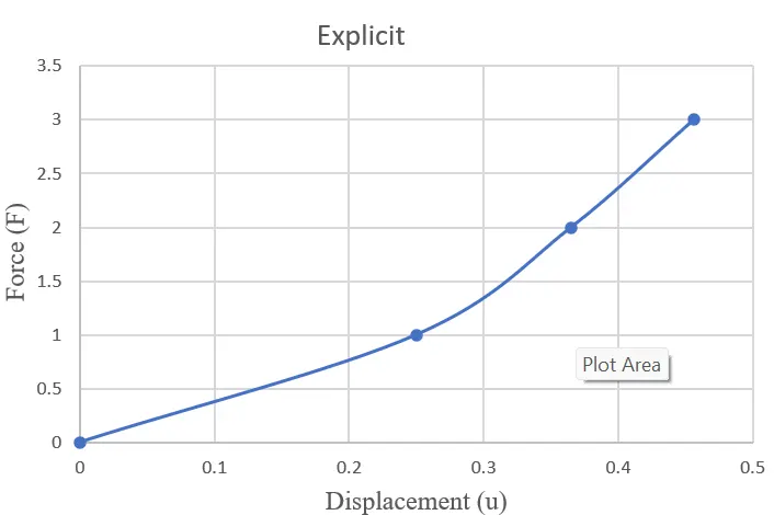
Table:1 Summary of explicit analysis results

Step i	∆Fi	∆ui	ui	(Fext)i	(Fint)i	(Fint)I - (Fext)I = R
1	1.0	0.25	0.25	1.0	1.578	0.578
2	1.0	0.115	0.365	2.0	2.707	0.707
3	1.0	0.091	0.456	3.0	3.790	0.790

From the above results external forces and internal forces are not in equlibrium because, F_int ≠ F_ext

Plot of force vs displacement in explicit results

(2) CALCULATION OF IMPLICIT METHOD TO SOLVE NON LINEAR DISPLACEMENT EQUATION

An implicit analysis is end of each step Newton-Raphson iterations are used to enforce equilibrium before moving to the next step.

Basically, an incremental force is applied to advance the solution forward at the beginning of a step. However, internal forces and external forces will not be in equilibrium unless the stiffness is linear for the

given step.

Hence, in order to achieve equilibrium, corrections must be made to the displacement.

This is accomplished by using Newton-Raphson iterations to minimize the residual, R(u) = fint − Fext.

Expanding the residual as a Taylor series about the current displacement u^j gives R^j+1 = R^j u^j +dR.(u^{j )}/du δu^j+1 +… = R^j + K(u^j) δu^j+1

By neglecting higher order terms in the series, setting R^j+1 = 0 and solving for δu^j+1 the following correction is obtained as, δu^{j +1} = −[k(u ^j )]^-1 . R^j

The iteration variable is j and it may take several iterations for the norm of the residual, ‖R‖ to be reduced below the chosen tolerance criteria.

Step 1 :

U₀ =0.0

The stiffness of the component is K(u) = df/du = 3u²+18u+4. -------(2)

substitute U₀ =0.0 value in equation (2) to we get

K(U₀) = 3(0)² + 18(0) + 4

K(U₀) = 4.

we know ∆F = 1 and the relationship is ∆F = k∆u-----(3)

Equation (3) can be rewritten as ,

∆F = K(U₀) .∆U1

∆U1 = ∆F / K(U₀)

= 1 / 4

∆U1 = 0.25.

U1 = U₀ + ∆U1

= 0 + 0.25

U1 = 0.25

F(u) = u³ + 9u²+4u

f_{int =} u₁³+9u₁²+4u₁

= (0.25)^{3 +}+9(0.25)²+4(0.25)

f_int = 1.578

Residual R⁰ = f_{int -} fext

=1.578 - 1

R⁰ = 0.578 which is greater than 0.01 as s result newton raphson method iterations are necessary.

Iteration -1

Calculating the new total correction to U_{1 =} U₁ ⁽⁰⁾

δ u^{( 1)} = −[k(u₁⁽⁰⁾ )]^-1 . R⁽⁰⁾

K(u₁) = 3u₁²+18u₁+4.

we know U1 = 0.25 ,

= 3(0.25)²+18(0.25)+4

K(u₁) = 8.6875

δ u^{( 1)} = −[k(u₁⁽⁰⁾ )]^-1 . R⁽⁰⁾

= - (8.6875)^-1 (0.578)

δ u^{( 1)} = - 0.0665

Therefore update value of u^{( 1)} is

u^{( 1)} = u₁⁽⁰⁾ + δ u^{( 1)}

= 0.25 - 0.0665

u^{( 1)} = 0.1834

Check residual again, fext = 1

f_{int = (}u₁¹ )³+9 (u₁ ^{1 )2}+4u₁¹

= (0.1834)³ + (9)(0.1834)² + (4) (0.1834)

f_int = 1.0432

Residual R^{( 1)} = f_{int -} fext

= 1.0432-1

R^{( 1)} = 0.0432 > 0.01 which means further newton raphson method iterations are necessary.

Iteration -2

Calculating the new total correction to U_{1 =} U₁ ⁽¹⁾

δ u^{( 2)} = δu₁ −[k(u₁⁽¹⁾ )]^-1 . R⁽¹⁾

Ku₁⁽¹⁾ = 3(u₁⁽¹⁾)² + 18(u₁⁽¹⁾) +4.

= 3(0.1834)² + 18( 0.1834 ) + 4

Ku₁⁽¹⁾ = 7.402

δ u^{( 2)} = δu₁ −[k(u₁⁽¹⁾ )]^-1 . R⁽¹⁾

= - (0.0665 ) - (0.0432)^-1 (0.0432)

δ u^{( 2)} = -0.0723

Therefore update value of u^{( 1)} is

u₁⁽²⁾ = u₁⁽⁰⁾ + δ u^{( 2)}

= 0.25 - 0.0723

u₁⁽²⁾ = 0.1776

Check residual again, fext = 1

f_{int = (}u₁² )³+9 (u₁ ^{2 )2}+4u₁²

= (0.1776)³ + (9)(0.1776)² + 4(0.1776)

f_int = 1.0006

Residual R^{( 2)} = f_{int -} fext

= 1.0006 - 1

R^{( 2)} = 0.0006 which is less than 0.01 which means newton raphson method iterations are not necessary.

so final value of u₁ ⁼ u₁⁽²⁾

u₁ = 0.1776

Step 2 :

u₁ = 0.1776

K(u₁) = 3u₁²+18u₁+4.

= 3(0.1776)² + 18(0.1776) + 4

K(u₁) = 7.291

we know ∆F = 1 and the relationship is ∆F = k∆u-----(3)

Equation (3) can be rewritten as ,

∆F = K(U₁) .∆U2

∆U2 = ∆F / K(U₁)

= 1 / 7.291

∆U2 = 0.137

U2 = U₁ + ∆U2

= 0.1776 + 0.137

U2 = 0.3147

Checking the residual,

fext = ∆F + ∆F = 2

f_{int =} u₂³+9u₂²+4u₂

₌ (0.3147)³ + 9(0.3147)² + 4(0.3147)

f_int = 2.181

Residual R⁰ = f_{int -} fext

=2.181 - 2

R⁰ =0.181 which is greater than 0.01 that means further newton raphson method iterations are necessary.

Iteration -1

Calculating the new total correction to U_{2 =} U₂ ⁽⁰⁾

δ u^{( 1)} = −[k(u₂⁽⁰⁾ )]^-1 . R⁽⁰⁾

K(u₂) = 3u₂²+18u₂+4.

We know u₂ = 0.3147

= 3(0.3147)² + 18(0.3147) + 4

K(u₂) = 9.9617

δ u^{( 1)} = −[k(u₂⁽⁰⁾ )]^-1 . R⁽⁰⁾

= -(9.9617)^-1 (0.181)

δ u^{( 1)} = -0.0182

Therefore update value of u₂^{( 1)} is

u₂⁽¹⁾ = u₂⁽⁰⁾ + δ u⁽¹⁾

= 0.3147 - 0.0182

u₂⁽¹⁾ =0.2962

Checking the residual again

fext = ∆F + ∆F = 2

_{fint= (}u₂¹ )³+9 (u₂ ^{1 )2}+4u₂¹

=(0.2962)³ + 9(0.2962)² + (4)(0.2962)

f_int = 2.00039

Residual R¹ = f_{int -} fext

= 2.00039 - 2

R¹=0.00039 < 0.01 which is less than 0.01 which means newton raphson method iterations are not necessary.

so final value of u₂ =u₂⁽¹⁾

u₂ ⁼ 0.2965

Step3 :

u₂ = 0.2965

K(u2) = 3u₂²+18u₂+4

=3(0.2965)² + 18(0.2965) + 4

K(u2) = 9.6007

we know ∆F = 1 and the relationship is ∆F = k∆u-----(3)

Equation (3) can be rewritten as ,

∆F = K(U₂) .∆U3

∆U3 = ∆F / K(U₂)

= 1 / 9.6007

∆U3 = 0.1041

U3 = U₂ + ∆U3

= 0.2965 + 0.1041

U3 = 0.4006

Checking the residual,

fext = ∆F + ∆F + ∆F = 3

f_{int =} u₃³+9u₃²+4u₃

= (0.4006)³ + 9(0.4006)² + 4(0.4006)

f_int = 3.116

Residual R⁰ = f_{int -} fext

= 3.116- 3

R⁰ = 0.116 which is greater than 0.01 that means further newton raphson method iterations are necessary.

Iteration -1

Calculating the new total correction to U_{3 =} U₃ ⁽⁰⁾

δ u^{( 1)} = −[k(u₃⁽⁰⁾ )]^-1 . R⁽⁰⁾

K(u₃) = 3u₃²+18u₃+4.

= 3(0.4006)² + 18(0.4006) + 4

K(u₃) = 11.683

δ u^{( 1)} = −[k(u₃⁽⁰⁾ )]^-1 . R⁽⁰⁾

= - (11.683)^-1 0.116

δ u^{( 1)} = -0.0092

Update the value of U_{3^{( 1)} =} U₃ ⁽⁰⁾ + δ u^{( 1)}

= 0.4006 - 0.00997

U_{3^{( 1)}} = 0.3911

Checking the residual again

fext = ∆F + ∆F + ∆F = 3

_{fint = (}u₃¹ )³+9 (u₃ ^{1 )2}+4u₃¹

= (0.3911)³ + 9(0.3911)² + 4(0.3911)

_fint = 3.0008

Residual R¹ = f_{int -} fext

= 3.0008- 3

R¹ = 0.0008 which is less than 0.01 that means newton raphson method iterations are not necessary.

so final value of U_{3^{( 1) =}} U₃

U₃ = 0.3906

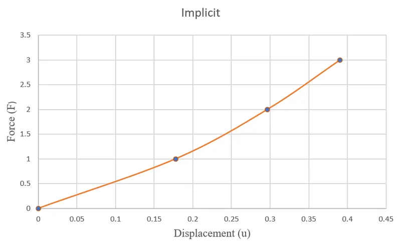
Table:2 Summary of implicit analysis results

Step i	∆Fi	∆ui	ui	(Fext)i	(Fint)i	(Fint)I - (Fext)I = R
1	1.0	0.25	0.1776	1.0	1.0006	0.0006
2	1.0	0.137	0.2965	2.0	2.0003	0.0003
3	1.0	0.1041	0.3906	3.0	3.0008	0.0008

From the above results external forces and internal forces are coming into equlibrium .

Plot of force vs displacement in implicit results

(3) CALCULATION OF EXACT SOLUTION OF THIRD ORDER POLYNOMIAL OF NON LINEAR DISPLACEMENT EQUATION

Take F(u) = u³ + 9u²+4u

u³ + 9u²+4u -F(u) = 0

F(u₁) = 1 ; u₁³+9u₁²+4u₁ -1 = 0 this equation is solved by using scientific calculator with polynomial degree 3 and to find out the value of u₁=0.1176

F(u₂) = 2 ; u₂³+9u₂²+4u₂ -2 = 0 this equation is solved by using scientific calculator with polynomial degree 3 and to find out the value of u₂=0.2961

F(u₃) = 3 ; u₃³+9u₃²+4u₃ -3= 0 this equation is solved by using scientific calculator with polynomial degree 3 and to find out the value of u₃=0.3910

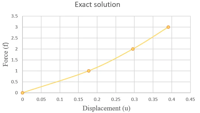
Table:3 Summary of exact solution results

Step i	ui
1	0.1776
2	0.2961
3	0.3910

Plot of force vs displacement in exact solution results

COMPARISON OF EXACT, EXPLICIT AND IMPLICIT RESULTS

S.NO	EXACT	EXPLICIT	IMPLICIT	Force
	ui	ui	ui	fi
1	0.1776	0.25	0.1776	1
2	0.2961	0.365	0.2965	2
3	0.391	0.456	0.3906	3

Plot of force vs displacement in both explicit and implicit results

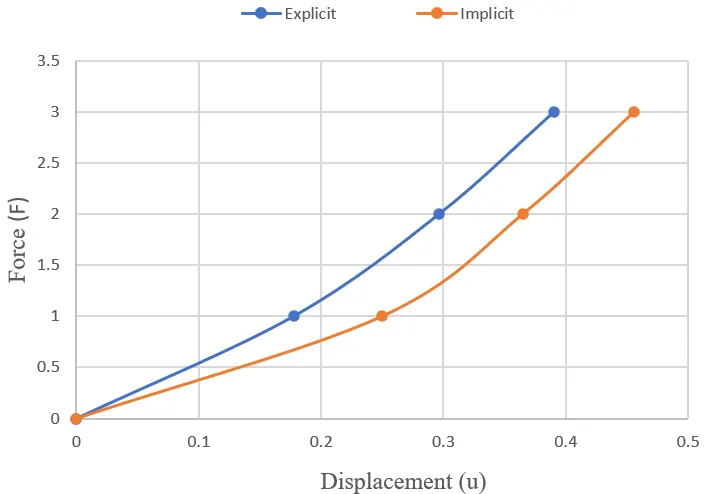
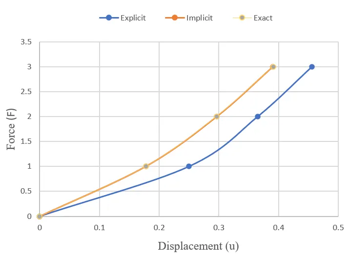
Plot of force vs displacement in implicit , explicit and exact solution results.

RESULT :

• From the comparison results, it is the evident from the plot explicit analysis drift from the exact solution but Explicit analysis results will not come closer to the exact solution.
• As we can see the implicit values are found more accurate and very close to the exact solution results which tell us that implicit method of calculation results are very accurate and close to the real values however implicit process is quite lengthy and more accuracy and more effort to solve than the explicit process.
• From the above plots we obtained implicit method give better solution comparing with the explicit method.
• The implicit method will equal to the exact solution due to newton raphton iteration used to enforce the equilibrium of external and internal forces.