Week - 2 - Explicit and Implicit Analysis

AIM: To solve the given `F(u)=u^3+9u^2+4u` using both the Explicit and Implicit analysis method with a tolerance of 0.001

OBJECTIVES:-

• A detailed report about Implicit and Explicit methods
• A complete calculation of the solving of the given equation and plotting the graphs of the results and a comparison between the two methods.

PROCEDURE:-

In static analysis, As we know that there is no effect of inertia (mass) or damping. But, In the dynamic analysis, nodal forces are associated with the mass/inertia, and damping is included.

We will use mainly two methods to solve the dynamic problems and they are

• Implicit method
• Explicit method

Explicit and implicit methods are used in numerical analysis for obtaining numerical approximations to solve solutions of time-dependent ordinary and partial differential equations which require computer simulations of physical processes.

Explicit method:

Explicit methods are used to calculate the state of the dynamic system at a later time from the state of the system at the current time, while explicit methods are used to find a solution by solving an equation involving both the current state of the system and the later one too.

In the explicit dynamic analysis, nodal accelerations of the model are solved directly (not inversely) as the inverse of the diagonal mass matrix times the net nodal force vector where net nodal force includes contributions from the exterior sources (such as body forces, applied pressure, contact, etc), element stress, damping, bulk viscosity, and hourglass control. once accelerations are known at time n, velocities are calculated at the time `n+frac1(2`, and the displacements are calculated at n+1. Now, from the displacements, we can calculate strain and from the strains, we can calculate the stresses, and the same procedure is repeated for every cycle.

The time step in the explicit analysis must be less than the Courant time step (the time it takes a sound wave to travel across an element).

Explicit methods should be used when the strain rate is equal to`10^-3` per second or more. These events can be illustrated by some examples such as an automotive crash, ballistic explosion, drop, and so on. In these cases, besides the variation of stress with strain, the rate of strain also needs to be considered. There are no convergence criteria to check or iteration. The solver focuses on the calculation of local finite element variables.

The solver calculates all of the local finite element variables for a given incrementation and moves to the next one. In the explicit method, the time step has to be super small. Otherwise, it’s impossible to pursue this equilibrium

Implicit method:

In Implicit analysis, each time increment has to converge, but users can set quite long time increments. In nonlinear implicit analysis, the solution of each step requires a series of trial solutions (iterations) to establish equilibrium within a certain tolerance. In explicit analysis, no iteration is required as the nodal accelerations are solved directly. Implicit transient analysis has no inherent limit on the size of the time step. As such, implicit time steps are generally several orders of magnitude larger than explicit time steps.

Implicit analysis requires a numerical solver to invert the stiffness matrix once or even several times over the course of a load/time step. This matrix inversion is an expensive operation, especially for large models. Explicit doesn't require this step.

Implicit methods should be used when the boundary conditions affect the structure slowly, and the effects of strain rates are minimum. Once the increment of stress as a function of strain can be established, geometry can be analyzed using implicit methods. The global equilibrium in the model is established in each time increment. This means each increment has to converge.

After global equilibrium is converged, the solver calculates all the local finite element variables (stresses, strain, etc.) for each increment. In the Implicit method, each time, increments are computed slowly and needed to get to the global equilibrium.

Explicit analysis handles nonlinearities with relative ease as compared to implicit analysis. This would include the treatment of contact and material nonlinearities.

SOLUTION

The given equation is

`F(u) = u^3+9u^2+4u` -------------------(1)

Now we have to solve the above equation using both Explicit and Implicit analysis with the tolerance of `10^-2`

We can calculate the stiffness of the bar by differentiating the given equation and we get

Stiffness of the bar `K(u) = frac(df)(du) =3u^2+18u+4` ----------------(2)

`triangleF= K triangleu`

(I) Explicit method

Step 1:

Take `u_o =0`

substituting `u_0` value in equation 2 we get `k(u_0) = 4`and take `triangleF=1`

Now we can calculate `triangle u_1= frac(triangle F)(k(u_o) )=frac(1)(4) =0.25`

Now `u_1=triangleu_1+u_0 = 0.25`

`F_(external)=triangleF=1`

`F_(Internal)= u_1^3+9u_1^2+4u_1 =1.5781`

Step 2 :

we have `u_1=0.25`

follow the same steps as discussed in the step 1, we get

`k(u_1) = 8.6875` and `triangle F =1`

`triangle u_2= frac(triangle F)(k(u_1) )=0.11510`

`u_2=triangleu_2+u_1 = 0.36510`

`F_(external)=triangleF+triangleF=2`

`F_(Internal)= u_2^3+9u_2^2+4u_2 =2.708`

Step 3:-

we have `u_2=0.36510`

Follow the same steps as discussed in step 2 , we get

`k(u_1) = 10.9718` and `triangleF=1`

`triangle u_2= frac(triangle F)(k(u_1) )=0.0911`

`u_3=triangleu_2+u_1 = 0.4562`

`F_(external)=triangleF+triangleF+triangleF=3`

`F_(Internal)= u_3^3+9u_3^2+4u_3 =3.7928`

It is evident from the results that external and internal forces are not in equilibrium as `F_(external) != F_(Internal`

The following table summarizes the results from the explicit analysis

Step i	`triangleF_i`	`triangle u_i`	`u_i'`	`(F_(ext))_i`	`(F_(Int))_i`	`R=(F_(Int))_i-(F_(ext))_i`
1	1	0.25	0.25	1	1.5781	0.5781
2	1	0.1151	0.3651	2	2.7080	0.7080
3	1	0.0911	0.4520	3	3.7928	0.7928

Implicit method:

Step 1:

`u_0=0`

`k(u_0)=4`and `triangleF=1`

`triangleu_1=frac(triangleF)(k(u_0) = 0.25`

`u_1=triangleu_1+u_0 = 0.25`

Now we have to check the Residual

`F_(external)=triangleF=1`

`F_(Internal)= u_1^3+9u_1^2+4u_1 =1.578`

`R^{0}= F_(Intenal)-F_(External)=0.5781`

`R^(0) > 10^-2=>` Newton-Raphson iterations are necessary

Calculate the correction value to `u_1=u_1^0`

`deltau_1=-[k(u_1^0)]^-1*R^0 = - (8.6875)^-1*0.578=-0.0665`

Now the updated `u_1^1=u_0^1+deltau_1 = 0.1835`

Again checking the residual

`F_(external)=triangleF=1`

`F_(Internal)= (u_1^1)^3+9(u_1^1)^2+4(u_1^1)=1.0432`

residual `R^1=F_(Internal)-F_(External)=0.432>10^-2=>` Newton-Rapshon iterations are necessary

Calculate the correction value to `u_1=u_1^0`

`deltau^2=deltau^1-[k(u_1^0)]^-1*R^1 = - 0.0723`

`u_1^2=u_0^1+deltau^2 = 0.1777`

Again checking the residual

`F_(external)=triangleF=1`

`F_(Internal)= (u_1^2)^3+9(u_1^2)^2+4(u_1^2)=1.0006`

Residual `R^1=F_(Internal)-F_(External)=0.0006<10^-2=>`Newton-Rapshon method is not necessary

Therefore the final value of `u_1=u_1^2=0.1777`

Step 2:

We have `u_1=0.1777`

`k(u_1)=7.2933`and `triangleF=1`

`triangleu_2=frac(triangleF)(k(u_1)) = 0.1371`

`u_2=triangleu_2+u_1 = 0.3148`

Now we have to check the residual

`F_(external)=triangleF+triangleF=2`

`F_(Internal)= u_2^3+9u_2^2+4u_2 =2.1822`

`R^0=F_(Internal)-F_(External)=0.1822>10^-2=>` Newton-Rapshon iterations are necessary

Calculate the corrected value to `u_1=u_1^0`

`deltau^1=-[k(u_1^0)]^-1*R^0 = - 0.0182`

The updated value of `u_2^1=u_2^0+deltau^1 = 0.2966`

Now we have to check the residual

`F_(external)=triangleF+triangleF=2`

`F_(Internal)= (u_2^1)^3+9(u_2^1)^2+4(u_2^1)=2.0042`

Reidual `R^1=F_(Internal)-F_(External)=0.0042<10^-2=>` Newton-Rapshon Iterations are not necessary

Therefore the final value of `u_2=u_2^1=0.2966`

Step 3:

we have `u_2=0.2966`

`k(u_2)=9.6027`and`triangleF=1`

`triangleu_3=frac(triangleF)(k(u_2)) = 0.1041`

`u_3=triangleu_3+u_2 = 0.4007`

Now we have to check the residual

`F_(external)=triangleF+triangleF+triangleF=3`

`F_(Internal)= u_3^3+9u_3^2+4u_3 =3.1121`

Residual `R^0=F_(Internal)-F_(External)=0.1121>10^-2=>`Newton-Rapshon iterations are necessary

Calculate the corrected value to `u_2=u_2^0`

`deltau^2=-[k(u_2^0)]^-1*R^0 = - 0.00958`

Now the updated value of `u_3^1=u_3^0+deltau^2 = 0.3911`

Now we have to check the Resisual

`F_(external)=triangleF+triangleF+triangleF=3`

`F_(Internal)= (u_3^1)^3+9(u_3^1)^2+4(u_3^1)=3.0008`

`R^0=F_(Internal)-F_(External)=0.0008<10^-2=>` Newto-Rapshon iterations are not necessary

So the final value of `u_3=0.3911`

The following table summarizes the results from the Implicit analysis

Step i	`triangleF_i`	`u_i'`	`(F_(ext))_i`	`(F_(Int))_i`	`R=(F_(Int))_i-(F_(ext))_i`
1	1	0.1777	1	1.0006	0.0006
2	1	0.2966	2	2.0042	0.0042
3	1	0.3911	3	3.0008	0.0008

It is evident from the results that external and internal forces are not in equilibrium as `F_(external) = F_(Internal`

Excat analysis:

step 1:

we have `F(u)=u^3+9u^2+4=1`

slovling aboue equation we get `u_1=0.1776`

Step 2:

we have `F(u)=u^3+9u^2+4=2`

solving above equation we get `u_2=0.2961`

Step 3:

we have `F(u)=u^3+9u^2+4=3`

solving above equation we get `u_3=0.3910`

The following table summarizes the results from the Implicit analysis

Step i	`u_i'`	`(F_(ext))_i`
1	0.1776	1
2	0.2961	2
3	0.3910	3

RESULTS AND PLOTS

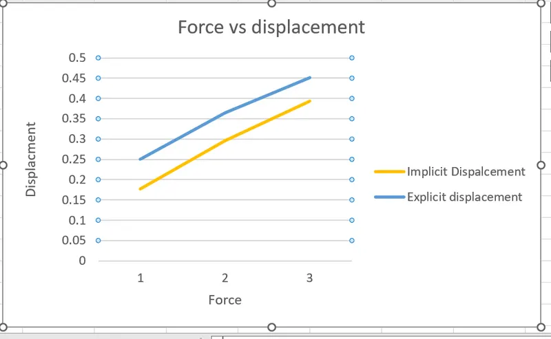
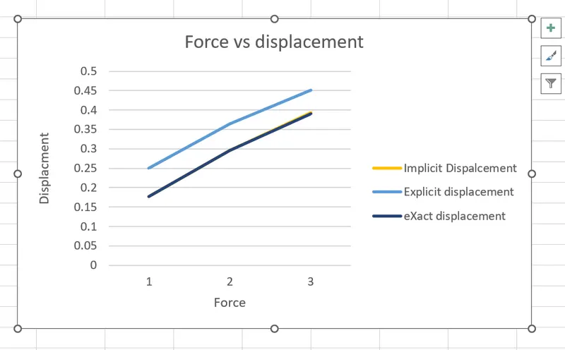
It is evident from the results that external and internal forces are not in equilibrium as `F_(external) = F_(Internal` in case of the Implicit method

CONCLUSIONS

• The implicit and Explicit numerical analysis is carried out for the given equation and the results are plotted for the comparision
• From the graphs, Implicit method is more accurate but time consuming and solemnly depends on the element size and time step whears the Explicit method deviates slightly form the exact result and needs more iteration to obtain a good result