Assignment 3-2D Element Formulation Challenge

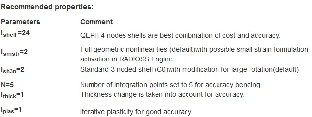
AIM: To run the simulation of the crash beam model ith base formulation followed by improved shell element properties (recommended properties).

OBJECTIVES:

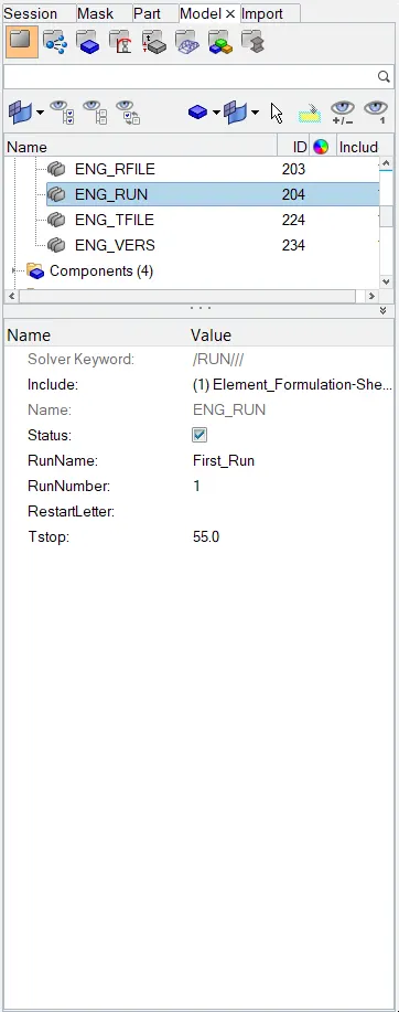
Objective 1. Using the crash beam file from the previous assignment, change the run to 55 ms.

• We can import the file to the radioss slover by >>import >> slover deck >> file >> import.
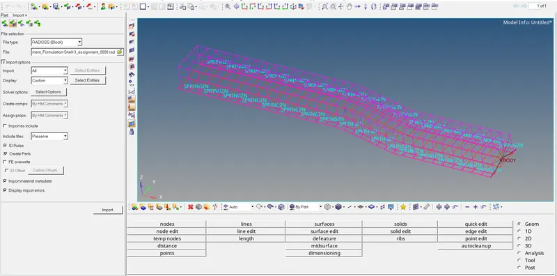
• Now we can change the run time to 55 ms by >>Model >>Cards >>ENG_RUN >>Tstop.
• 

Objective 2. Change the number of animation steps during the simulation to a minimum of 25 and a maximum of 60.

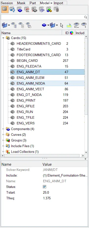
• In the property section, we can the Tstart value to a minimum of 25 and accommodate a maximum of 60 animation steps with a Tfreq value of 1.375. because I selected 40 in between 25 and 60 and for tfreq we have to divide Tstop with the selected number.
• >>Model >>cards >>ENG_ANIM >>Tstart >>Tfreq.

Objective 3. Run the base simulation without any modification to element properties.

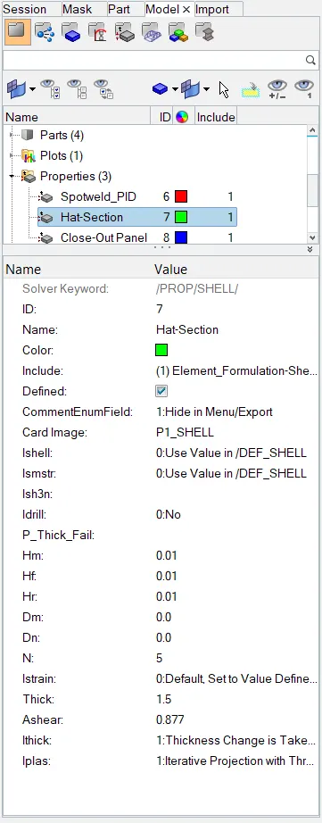
Properties for base simulation

• we can run the simulation >>analysis>>radioss
• we have to save the file in the new folder to store all output files. In the options tab, we have to recommend keeping "-nt4" which indicates 4 crores to run the simulation faster. where "nt" indicates a number of threads.

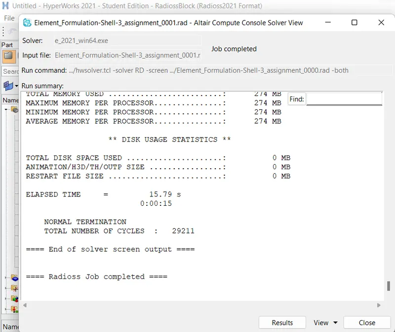
Analysis is done

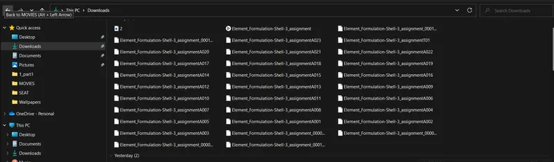
Files created after simulation

• now the simulation is done and a number of output files are created as shown. after simulation, now we have to visualize the results for visualization we need to shift from hyper mesh to hyper view tab.
• view>>browsers>>hyperview. in this way we can select the hyper view tab.

accessing the hyper view

• After accessing the hyper view, we should input the simulation file. for this, we have to use the h3d file that was generated when RADIOSS processed the starter file.
• It is generated in the files which are shown above. After selecting it, we can just simply click "apply".

Opening h3d file in hyper view

• Doing so many generations the simulation animation. we can change what is given by simulation by selecting the "contour" option in the toolbar for our required parameters.

Objective 4. At the end of the simulation, do the energy error and mass error checks and determine whether would be acceptable.

• After the simulation results are obtained, now we have to calculate the energy error and mass errors. The errors can be found by opening the 0000.out file, in the notepad, as shown below.

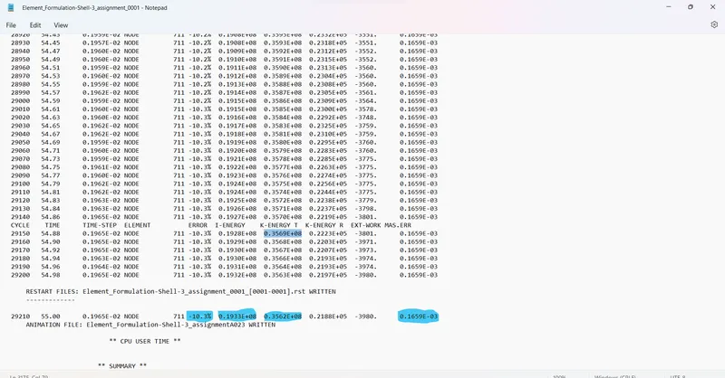
engine ouput file for default parameters

• The energy error is -10.3%. Internal energy = 0.1932E+08 gm^2/sec^2 and kinetic energy = 0.3563E+08 gm^2/sec^2. and mass error is 0.16593E-03
• the acceptable tolerance for energy error is -15% to +5%.

Objective 5. If acceptable, plot Rigid wall forces, internal energy, hourglass energy, contact energy, and total energy of the simulations.

• as seen the energy and mass error are within the acceptable tolerance level. so no\w we can go ahead and plot the graphs. For plotting we have to open Hyperview2D.

Opening the Hyperview2D

• In the Hypergraph section, we need to import a file. For this, we will be using the result output file by the RADIOSS slover which is in the "T01 file"

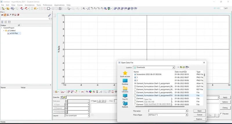
importing the TO1 file

• Select the required options as shown below to plot all the graphs.

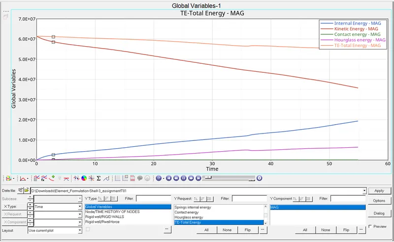
graphs formed by default properties

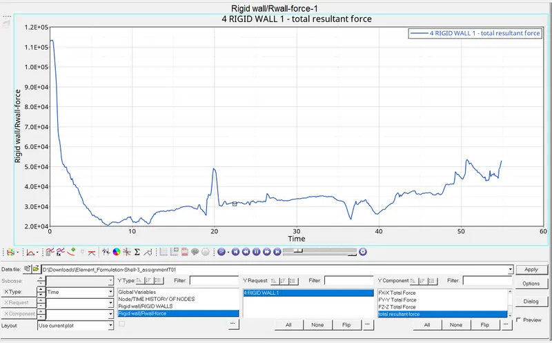
Total resultant force by Default properties

Objective 6. Change all the shell elements' properties to recommended properties, save this as separate, rad files and run the simulation.

• Now we have to carry out the simulation for the recommended properties. We can repeat the process of importing the original slover deck file and change the values of Tstop= 55ms; Tstart= 25 and Tfreq= 1.375 in the slover tab of the imported file.
• Now we can edit the properties as follows >>Model>>properties>>hat-section(Select the required properties)>>close-out panel(select remaining properties).

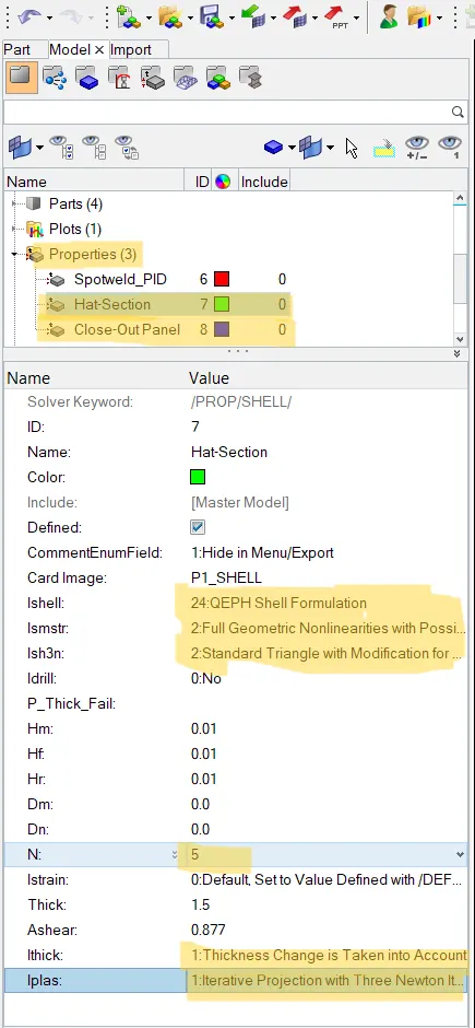
Recommended properties

• Now we have to run the simulation again and store all the output files in a different folder. And for simulation, we can proceed with the same procedure as discussed above.
• After that, we can switch to hyper view to generate the simulation as processed before.

Objective 7: Follow objectives 5 and 6

• the next procedure is to check the obtained values for internal energy, total energy, and mass error from the engine output file named 00001.0ut.

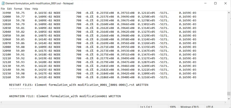
• As we can observe, there is a drastic reduction in the energy error, as we are evident in the more natural-looking simulation. Earlier the hourglass energy is -10.3% and now it was reduced to -0.1% which is almost equal to zero and the error in the mass is 0.1659E-03 %.
• whereas in the recommended property which is QEPH-4 the hourglass energy is zero because the property of the element has improved with 4 noded integration points and it has physical hourglass stabilization property. Thus it avoids the hourglass completely in this case.
• Now we can generate the graphs.

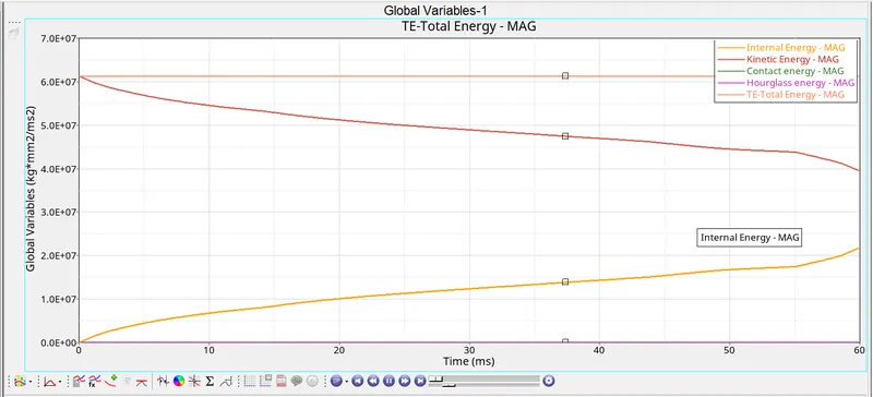
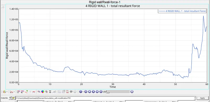
Objectives 8 and 9:Create a brief report comparing all the results from step 5 and step 6 for both simulations & Comment on whether there is any change in the results and why there is any change in the result.

• we can open plots of the two cases as shown below by multiplot selector, which makes comparison easy.

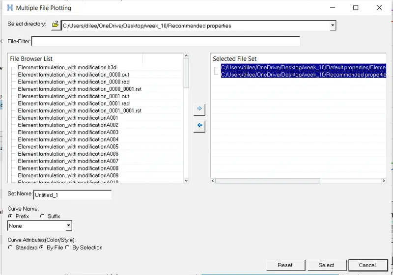
Multiplot selecting

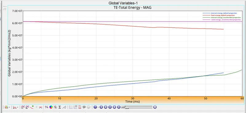
Energy comparison

• The major difference in both simulations is the reduction in hourglass energy. so, the introduction of QEPH shell formulation(Ishell=24) provides an artificial stiffness to the shell elements and helps counter hourglass formulation.
• Therefore, the simulation with RECOMMENDED PROPERTIES simulation is looking more natural than the default properties simulation.

Attribute	Default properties	Recommended properties
Energy error	-10.3%	-0.1%
Mass error	0.1659E-03 %	0.1659E-03 %
Internal energy	0.1932E+08	0.2186E+08
Kinetic energy	0.3563E+08	0.3940E+08
Hourglass energy	Hourglass energy increases over time, as there is no physical stabilization in default properties	Hourglass energy is zero. because of having all the physical properties
Total energy	Total energy decrease with time because of hourglass energy	Absence of Hourglass energy, the total energy almost remains constant with time.