Challenge

Assignment 4-RADIOSS Material Laws Challenge

KKuruba Dileep Kumar8 Jun 2022

AIM:- To perform the crash analysis on the given model of the stater files and compare the results for different cases by applying the material laws which are available in the Radioss.

Objective:-

To carry out the simulations for the given starter files and compare the results of the different cases by applying material laws. The given input starter files are FAILUTRE_JHONSON_0000.rad and LAW27_0000.rad. The laws applied to the starter files are :

LAW 1 - FAILURE_JHONSON_0000.rad - basic simulation
LAW 1 - FAILURE_JHONSON_0000.rad - with ifail_sh=1;Dadv=1;lxfem=1
LAW 1 - FAILURE_JHONSON_0000.rad - with fail/JHONSON card deleted
LAW 1 - FAILURE_JHONSON_0000.rad - with EPS_p_max card deleted
LAW 1 - FAILURE_JHONSON_0000.rad - with fail/JHONSON card deleted and assigning the given properties
LAW27 - LAW27_0000.rad -with recommended properties
LAW27 - LAW27_0000.rad - with recommended shell properties and given preference curve.

THEORY:

ISOTROPIC ELASTICITY LAW (LAW 1)

Isotropic means the properties of the material are elements are identical in all directions
Elasticity is the ability of a deformed material body to return to its original shape and size when the forces causing the deformation are removed
Radioss provides two different types of elasticity and they are "Linear Elastic" and Hyper-Elastic"
Law 1 should not be used for the parts are elements undergoing large deformation
For large deformation, the of elements yield law can be used.

JHONSON-COOK LAW (LAW 2)

Jhonson-cook law represents isotropic elastoplastic material.
The Johnson-Cook model is a function of von mises tensile flow stress, in accordance with strain hardening, strain rate hardening, and thermal softening.
In the material card of Law 2, we have an option known as EPS_max which indicates the strain at the failure.
/FAIL/JHON card gives more commands to the user on the failure of the element of the jhonson-cook strain.

ELASTOPLASTIC MATERIAL WITH BRITTLE FAILURE (LAW 27)

In this model failure or damage to the elements occurs in tension loading
The major drawback of Law 27 is it limits only shell element
This law came more existence for modeling the brittle glass materials.

PROCEDURE:

Case 1:-

Go to the hyper works and import the file as >>menu>>import>> slover deck >>browse and import the file
For case 1 the FAILURE_JHONSON_0000.rad model is imported.

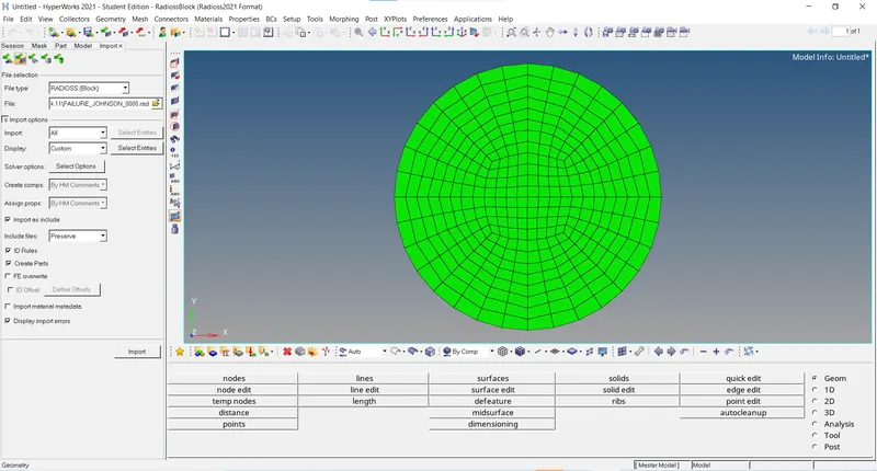
FAILURE_JHONSON_0000.rad file is imported

we can check the units of the starter file by opening the begin card in the session tab. and The standard units are checked with the LS Dyna website.
In the base simulation, we have to run the simulation with the default values. so we are recommended to don't change any values

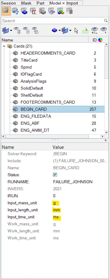
Units check with BEGIN_CARD

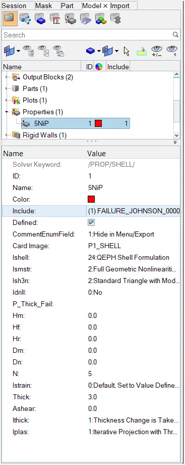
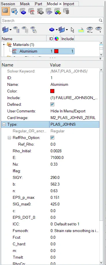
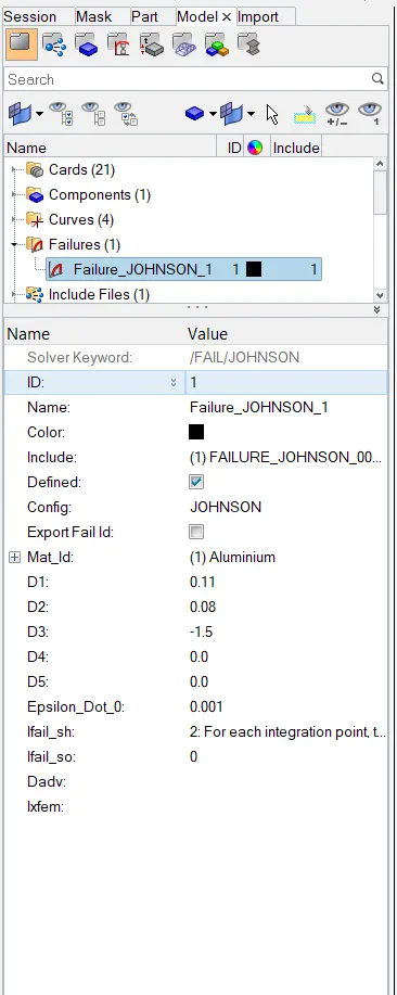
Default values of properties, failure and material cards

we can run the simulation >>analysis>>radioss
we have to save the "file as LAW2_epsmax_failure_0000.rad" in the new folder to store all output files. In the options tab, we have to recommend keeping "-nt4" which indicates 4 crores to run the simulation faster. where "nt" indicates a number of threads.

Destination for output files

After clicking Radioss, the analysis window pops up and we can see after a few minutes the job was done successfully.

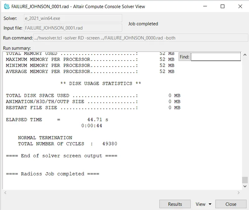
analysis was done successfully

The simulation is done, now we have to visualize it in hyper view. for this we have to open hyper view and import the .h3d file.
and opening contour, then select von misses and averaging method as a simple average method.

Simulation of case 1

In the next step, we have to carry out the energy and mass error analysis. For this, we have to 0001.out file in the notepad. Scrolling to the end we can see the energy error and mass error.

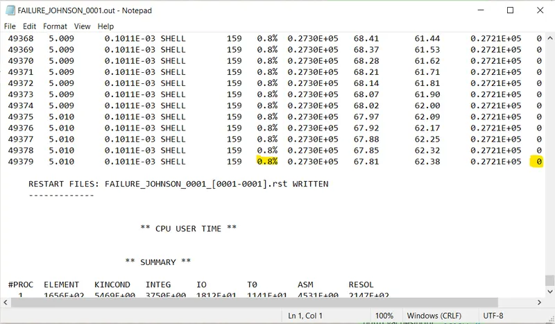
energy and mass error

The final energy is 0.8%, which is very acceptable and there is no mass error.
Now we have to plot the graphs in the hypergraph tool and in hypergraph we have to import the.T01 file.

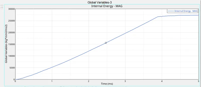
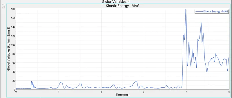
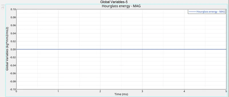
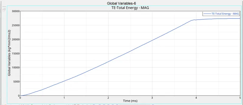
From the above graphs, internal energy first increases with time but after some time remains constant.
we have taken the QEPH element shell, so the hourglass energy is equal to zero.
Total energy first increases with time but after some time remains constant.

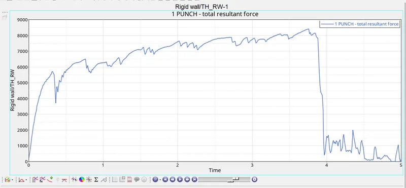
Rigid wall forces are the forces acting on the rigid wall. for this case wall is moving, so, to move any object some external force is necessary that the reason the rigid wall forces start to increase from zero. once the motion is achieved the force starts to decrease.

Case 2:-

For case 2 also, import the FAILURE_JHONSON_0000.rad as previously.
Now, We have to make some changes to the fail/JHONSON card, which can be accessed from the Model tab of the failure card.
Now we have to change ifail_sh = 1, which determines the shell failure method.
lxefm =1, which allows failed element to cracked not deleted.
Dadv=1 gives the criteria for how much an element can break into small pieces. If it goes beyond the limit the element gets deleted.

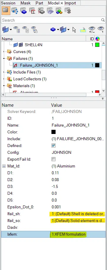
Failure card properties are changed

Now run the analysis and save the file name as "Law2_eapmax_crack_0000.rad" with connectors turned on and options as -nt4. and run the simulation as in the previous case.

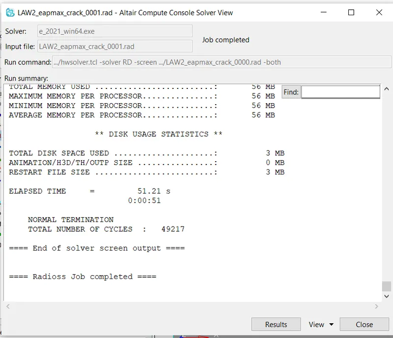
Abalaysis was done successfully

Now we have to carry out energy and mass error same as the previous case.

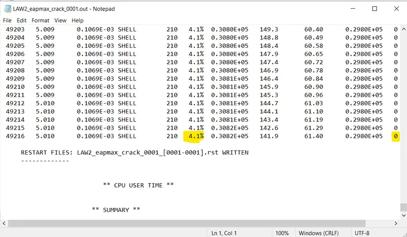
The energy error is 4.3% and the mass error is 0.00%. the energy error is less than 5% which is acceptable, we can go ahead to plot graphs in the hypergraph.

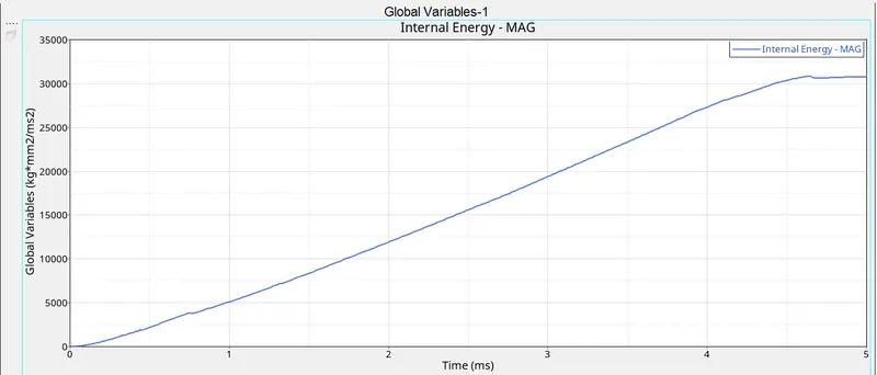
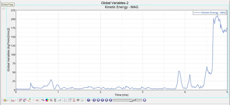
From the above graphs, internal energy first increases with time but after some time remains constant.
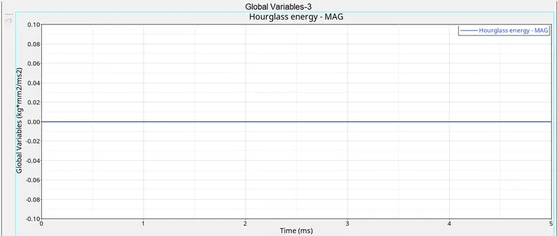
we have taken the QEPH element shell, so the hourglass energy is equal to zero.
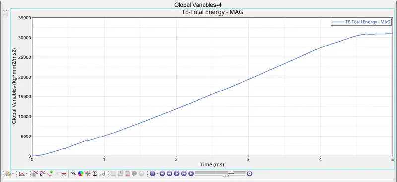
Total energy first increases with time but after some time remains constant.

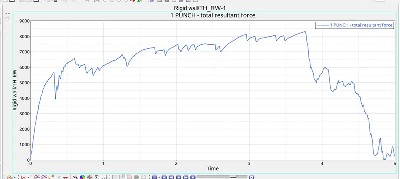
Rigid wall forces are the forces acting on the rigid wall. for this case wall is moving, so, to move any object some external force is necessary that the reason the rigid wall forces start to increase from zero. once the motion is achieved the force starts to decrease.

Case 3:-

Now import the "Law2_eapmax_crack_0000.rad" into the HyperWorks slover deck, which was created in case 2.
for this case, we have to delete the fail/JHONSON card. for this >>Model>>failures>>fail/JHONSON( then delete).

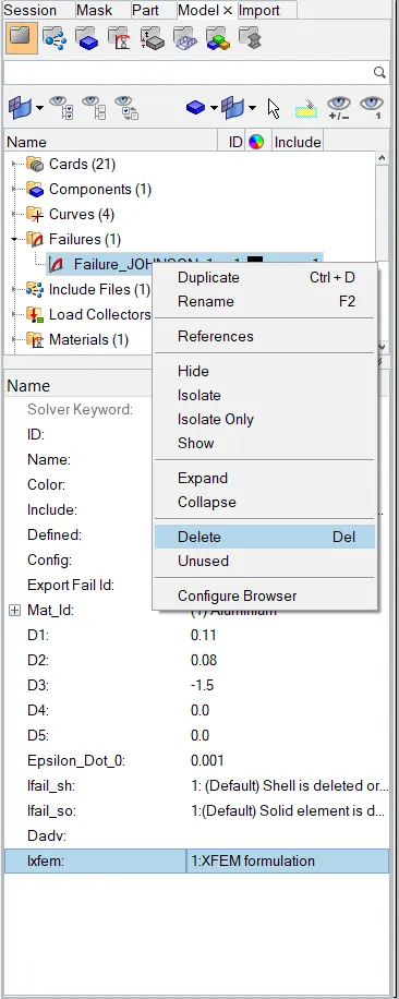
Deletion of fail/JHONSON card

Now run the analysis and save the file as LAW2_epsmax_nofail_0000.rad.
After the completion of the simulation, visualize the simulation in the hyper view tab

Now we have to check energy and mass errors from the output 0001.out file in the notepad.

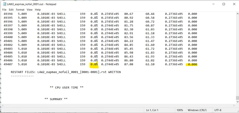
The final energy error is 0.8% which is less than 5% and acceptable and there is no mass error
so we can proceed to plot the graphs in the hyper view by opening the T01 file.

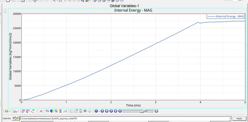
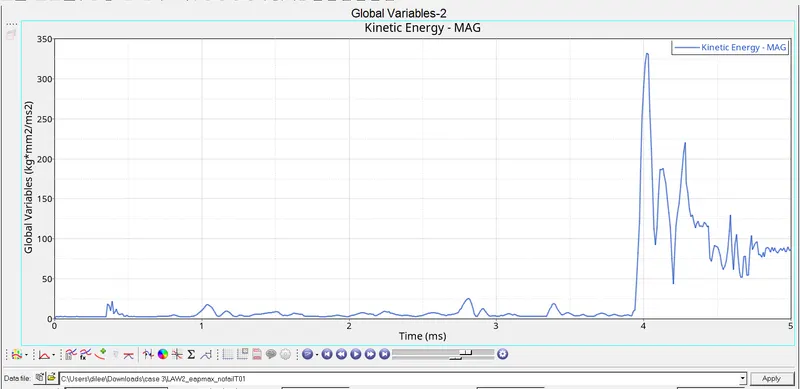
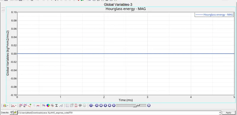
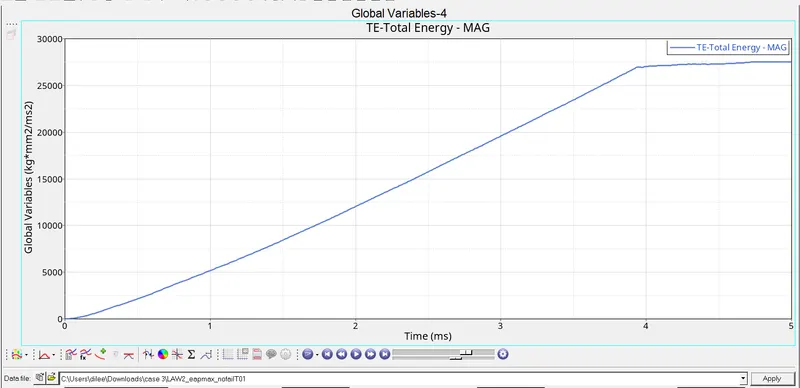
From the above graphs, internal energy first increases with time but after some time remains constant.
we have taken the QEPH element shell, so the hourglass energy is equal to zero.
Total energy first increases with time but after some time remains constant.

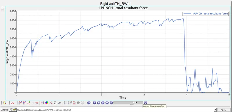
Rigid wall forces are the forces acting on the rigid wall. for this case wall is moving, so, to move any object some external force is necessary that the reason the rigid wall forces start to increase from zero. once the motion is achieved the force starts to decrease.

Case 4:-

In this case, we have to import the case 3 input fail "LAW2_epsmax_nofail_0000.rad".
This time, we have to delete the EPS_P_max value (making the value zero). This can be achieved by >>model>>materials>>EpPS_P_max(make zero).

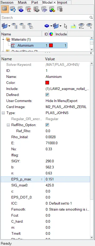
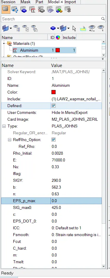
Making EPS_P_max equal to zero

After this, we can go to the analysis tab of Radioss. Then save the file as "LAW2_0000.rad". Same procedure as followed as in case 1.
After the analysis, ae can switch to the hyper view tab to visualize the simulation by importing the .h3d file.

Now we have to check the energy error and mass error by opening the 00001.out file.

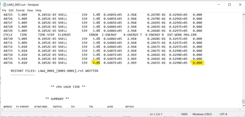
The final energy error is 3% which is less than 5% and acceptable and there is no mass error
so we can proceed to plot the graphs in the hyper view by opening the T01 file.

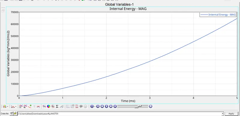
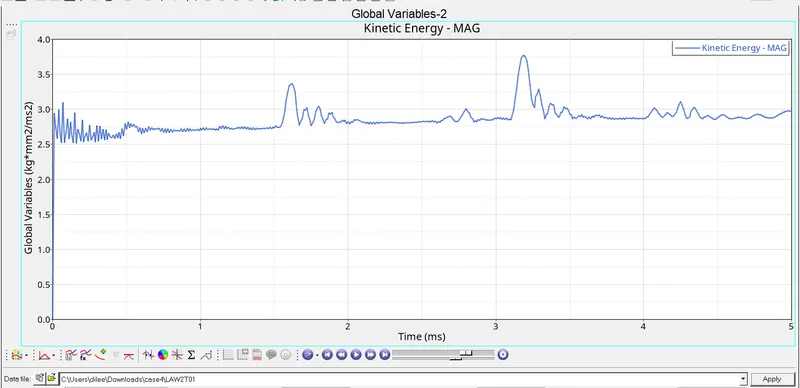
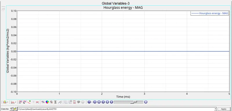
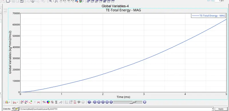
From the above graphs, internal energy increases with time.
we have taken the QEPH element shell, so the hourglass energy is equal to zero.
Total energy increases with time.
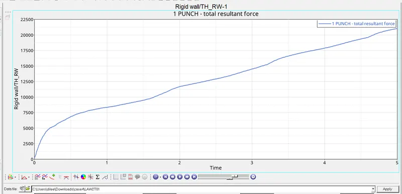
Rigid wall forces are the forces acting on the rigid wall. for this case wall is moving, so, to move any object some external force is necessary that the reason the rigid wall forces start to increase from zero.

Case 5:-

In this case, import the original starter file of case 4
Open the material card and change the card image to law1 by keeping the same values of young modulus, density, and poisons ratio.

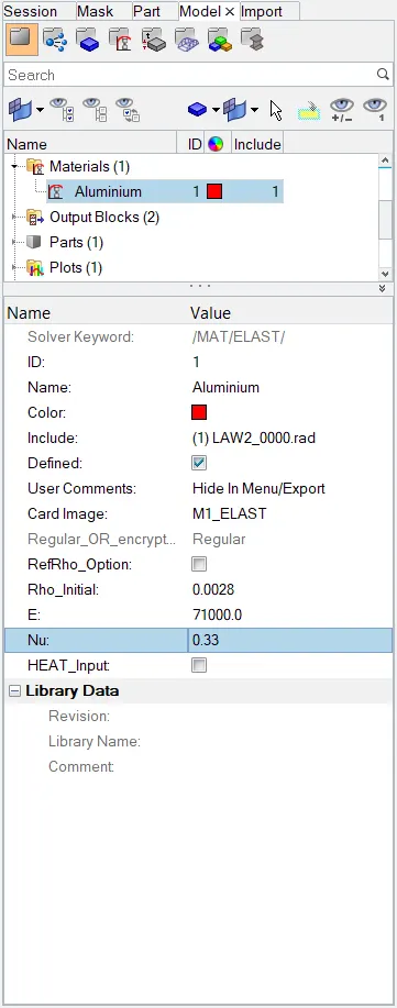
Now shift to the analysis tab for analysis and save the file as "LAW1_0000.rad". then click the Radioss for simulation
After the completion of the simulation, shift to the hyper view tab and import the h3d file to visualize the simulation.

Now we have to check energy and mass errors from the output 0001.out file in the notepad.

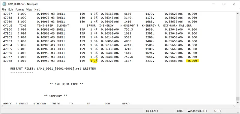
The energy error is 1.3% and the mass error is 0.00%. the energy error is less than 5% which is acceptable, we can go ahead to plot graphs in the hypergraph.

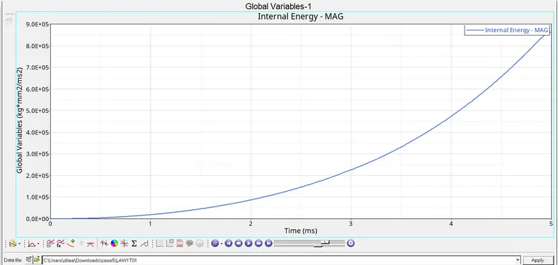
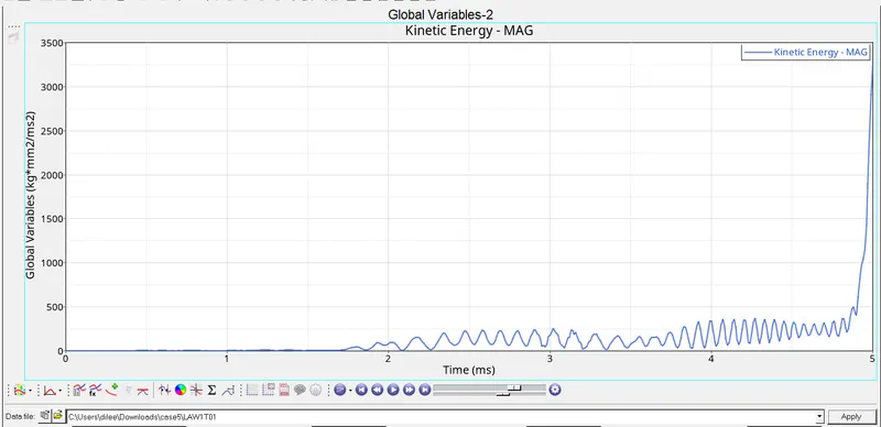
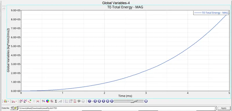
From the above graphs, internal energy increases with time.
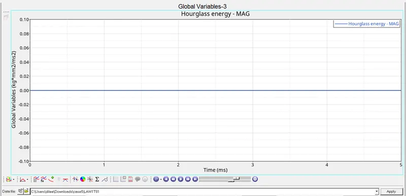
we have taken the QEPH element shell, so the hourglass energy is equal to zero.
Total energy increases with time.

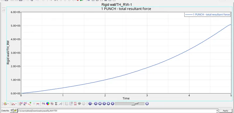
Rigid wall forces are the forces acting on the rigid wall. for this case wall is moving, so, to move any object some external force is necessary that the reason the rigid wall forces start to increase from zero.

Case 6:-

In this case, we have to import the case 1 file named LAW2_epsmax_Failure_0000.rad".
we have to perform the simulation for Law 36 material card similar to case 5.

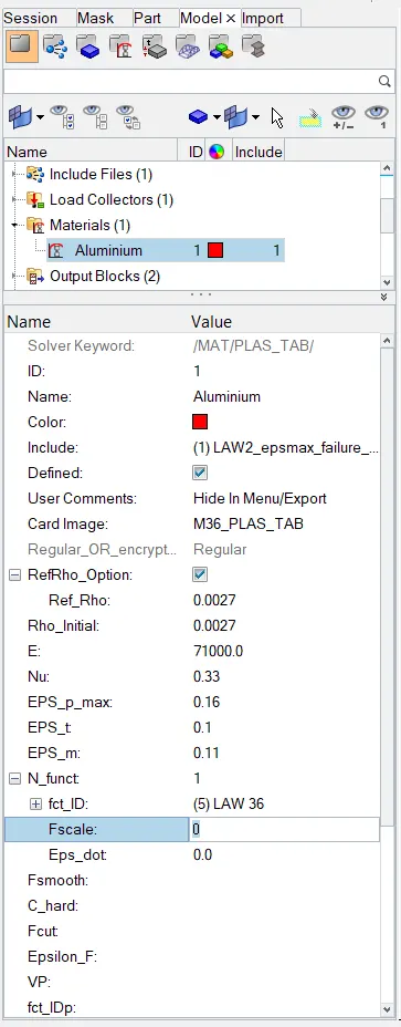
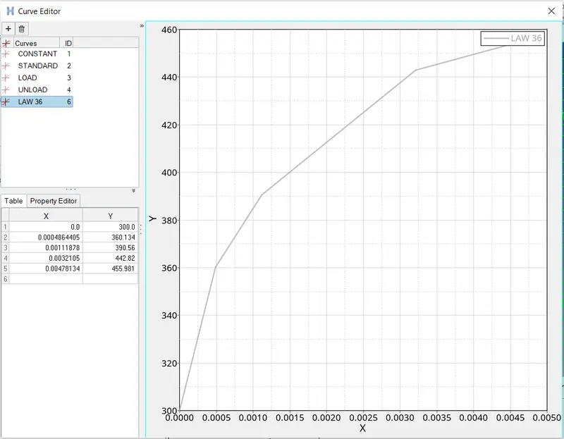
We can create a new curve named as Law 36 by >>Right click on model tab >>create>>curve>> give X and Y coordinate values

we can run the simulation >>analysis>>radioss
we have to save the "file as LAW36_0000.rad" in the new folder to store all output files. In the options tab, we have to recommend keeping "-nt4" which indicates 4 crores to run the simulation faster. where "nt" indicates a number of threads.
Now shift to the analysis tab for analysis and save the file as "LAW1_0000.rad". then click the Radioss for simulation
After the completion of the simulation, shift to the hyper view tab and import the h3d file to visualize the simulation

Now we have to check energy and mass errors from the output 0001.out file in the notepad.

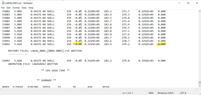
The energy error is -0.8 % and the mass error is 0.00%. The acceptable range for error is -15% to 5% which is acceptable, we can go ahead to plot graphs in the hypergraph.

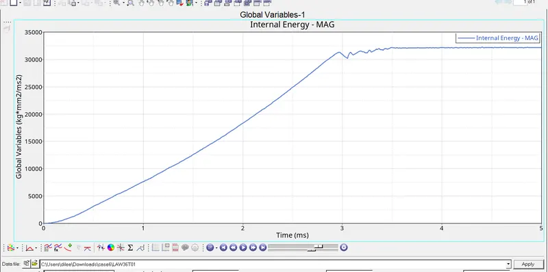
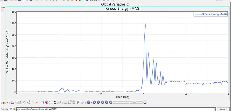
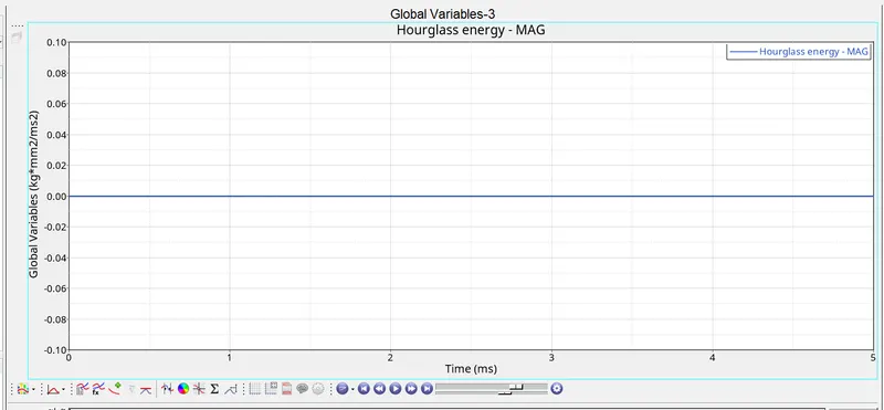
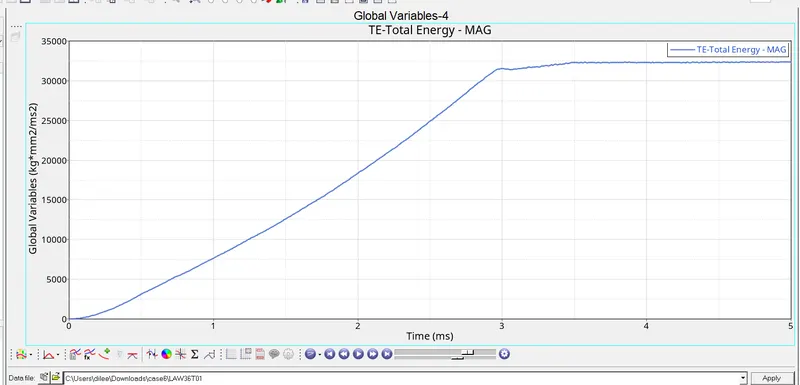
From the above graphs, internal energy first increases with time but after some time remains constant.
we have taken the QEPH element shell, so the hourglass energy is equal to zero.
Total energy first increases with time but after some time remains constant

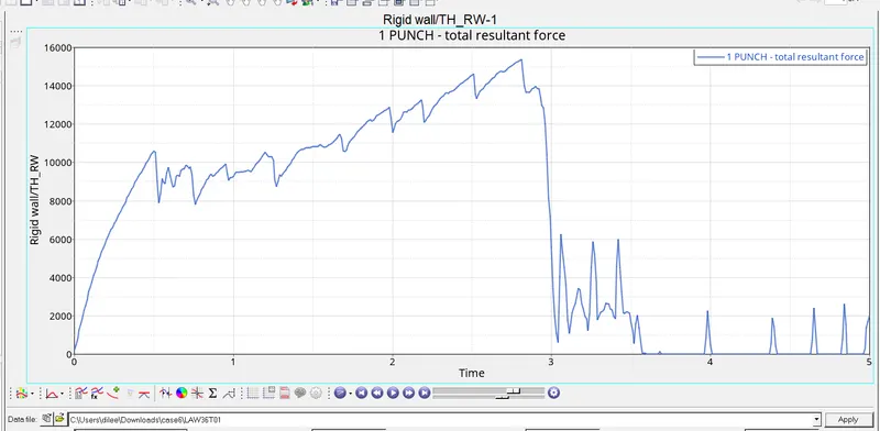
Rigid wall forces are the forces acting on the rigid wall. for this case wall is moving, so, to move any object some external force is necessary that the reason the rigid wall forces start to increase from zero.

Case 7:-

For this case, we have open, LAW27_0000.rad file
We have to perform the simulation with the Law 27 material card as discussed in the previous cases.

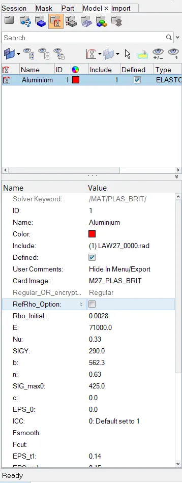
we can run the simulation >>analysis>>radioss
we have to save the "file as LAW36_0000.rad" in the new folder to store all output files. In the options tab, we have to recommend keeping "-nt4" which indicates 4 crores to run the simulation faster. where "nt" indicates a number of threads.
Now shift to the analysis tab for analysis and save the file as "LAW27_0000.rad". then click the Radioss for simulation
After the completion of the simulation, shift to the hyper view tab and import the h3d file to visualize the simulation

Now we have to check energy and mass errors from the output 0001.out file in the notepad.

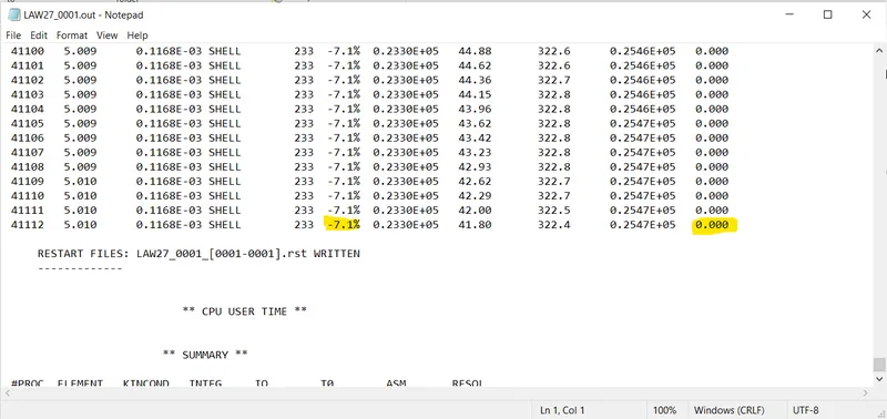
The energy error is -7.1 % and the mass error is 0.00%. The acceptable range for error is -15% to 5% which is acceptable, we can go ahead to plot graphs in the hypergraph.

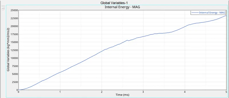
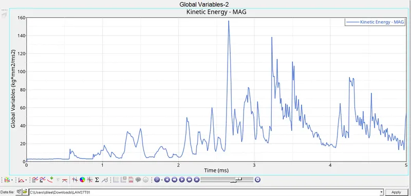
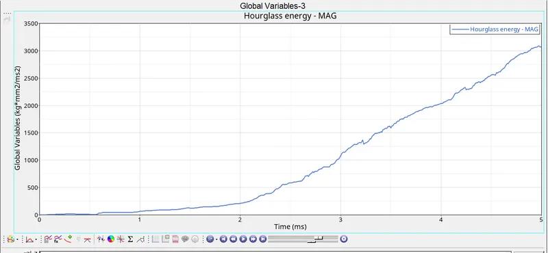
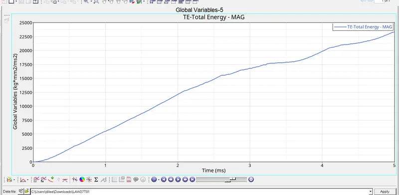
From the above graphs, internal energy first increases with time but after some time remains constant
Total energy first increases with time but after some time remains constant

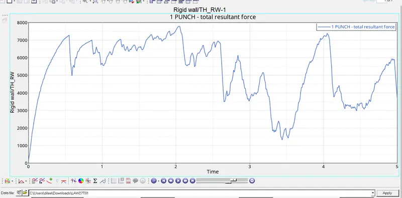
Rigid wall forces are the forces acting on the rigid wall. for this case wall is moving, so, to move any object some external force is necessary that the reason the rigid wall forces start to increase from zero.

Comparison of 7 cases

Case no	Total No. of cycles	ENERGY ERROR (%)	MASS ERROR(%)	SIMULATION TIME (sec)	Elements After impact
1	49380	0.8	0	45.37	Deleting after deformation beyond the limit
2	49217	4.1	0	51.21	Deleting after deformation beyond the limit
3	49408	0.8	0	66.97	Deleting after deformation beyond the limit
4	48737	3	0	47.05	Deforming but not deleting
5	47969	1.3	0	57.82	stretching
6	53094	-0.8	0	49.70	Deleting after deformation beyond the limit
7	41113	-7.1	0	39.61	Deleting after Failing

Learning Outcomes

Learned different types of material cards
learned about failure cards in hyper mesh
and learned about rigid wall forces and different energies.
comparison between different cases with different material cards

Assignment 4-RADIOSS Material Laws Challenge

Ship work like this
in your own course.

Talk to a career counsellor

Ship work like thisin your own course.

Talk to a career counsellor

Ship work like this
in your own course.