Week - 2 - Explicit and Implicit Analysis

AIM:

To solve the given equation `F(u)=u^3+9u^2+4u` by using both implicit and Explicit methods with a tolerance of `10^-2`

EXPLICIT AND IMPLICIT ANALYSIS:

There are two types of approach here Implicit and Explicit, this is used to solve the finite element analysis problems. Implicit and Explicit analysis differ in the approach to time incrementation. In Implicit analysis, each time increment has to converge for eg., Static structural, Harmonic, Modal analysis, etc., but you can set pretty long time increments. Explicit on the other hand doesn't have to converge each increment, but for the solution to be accurate time increments must be super small eg., Crash, Blast, and Impact.

>>> EXPLICIT:

In explicit dynamic analysis, nodal accelerations are solved directly(not iteratively) as the inverse of the diagonal mass matrix times the net nodal force vector where net nodal force includes contributions from exterior sources (body forces, applied pressure, contact, etc.,), element stress, damping, bulk viscosity, and hourglass control. Once acceleration is known at time n, velocity is calculated at a time `n+1/2`, and displacement at a time `n+1`. From displacement comes strain, From strain comes stress, and the cycle is repeated. In explicit analysis, no iteration is required as the nodal accelerations are solved directly.

`n Non-linear problems, those with large deformations and/or nonlinear material response, the highest frequency of the model will continually change, which consequently changes the stability limit. Explicit has two strategies for time incrementation control, fully automatic time incrementation (where the code accounts for changes in the stability limit) and fixed time incrementation.

LS DYNA is one of the software which is used to solve the explicit analysis problem for Crash, Impact, Penetration, etc.,

ABAQUS & PAMCRASH are also used for explicit analysis problems.

>>> IMPLICIT:

In Implicit analysis, the displacement is not a function of time(i.e, x= Constant), hence the velocity and accelerations which are time derivations of displacement turn out to be zero, mass and damping factorscan can be neglected, the implicit method based on network method, Newton Raphson method, Inversion of the stiffness matrix is required. Static analysis is done using an implicit solver in LS DYNA. Dynamic analysis can be done via the explicit or the implicit solver.

In Non-linear implicit analysis, the solution of each step requires a series of trial solutions (iterations) to establish equilibrium within a certain tolerance, implicit analysis requires a numerical solver to invert the stiffness matrix once or even several times over the course of a load/time step. This matrix inversion is an expensive operation, especially for large models.

Implicit methods are mainly used in software like ANSYS, ABACUS, NASTRAN, etc.,

EXPLICIT ANALYSIS:

If the nonlinear force versus displacement relationship is not known, but the stiffness is known, it is possible to construct the graph of force versus displacement numerically

It can be done using an increment explicit load control scheme

The following equation is solved using the explicit method as follows,

`F(u)=u^3+9u^2+4u` --------(1)

Use this equation and solve using both Explicit and Implicit methods that have tolerance of `10^2`

Differentiating force with a request to displacement gives the stiffness (k) of the bar (since F=kx)

`k(u)=(df)/(du) = 3u^2+18u+4` ---------(2)

Variables are as given below;

• `U=Displacement`
• F = External force
• K = Stiffness
• `Deltau=` Incremental Displacement
• `DeltaF=` Incremental externally applied force

Here, three equal load increments (or steps) of `Delta F=1` unit of each used to load the tension ba

>>>Step 1:

`u_0=0`

`k(u_0)=3(0)^3+18(0)^2+4(0) = 4`

Now,

`Deltau_1 = (Deltaf)/(k(u_0)) =1/4 = 0.25`

`u_1=u_0+Deltau_1 = 0.25`

`F_(External) = DeltaF=1;`

`F_(Internal)=u_1^3+9u_1^2+4u_1=(0.25)^3+9(0.25)^2+4(0.25)=1.5781`

`R=F_I-F_E=1.5781-1=0.5781`

>>>Step 2:

Put `u_1=0.25`

`k(u_1)=3(0.25)^2+18(0.25)+4 = 8.6875`

Now,

`Deltau_2=1/8.6875 = 0.1151`

`u_2=u_1+Deltau_2=0.1150+0.25 = 0.3651`

`F_(External) = DeltaF+DeltaF=1+1=2`

`F_(Internal)=u_2^3+9u_2^2+4u_2=(0.25)^3+9(0.25)^2+4(0.25)=2.7087`

`R=F_I-F_E=2.7087-2=0.7087`

>>>Step 3:

Put `u_2 = 0.3651`

`k(u_2)=3(0.3651)^2+18(0.3651)+4 = 10.9713`

`DeltaF=1,`

`Deltau_3=1/10.9713 = 0.0971`

`u_3=u_2+Deltau_3=0.3651+0.09176 = 0.4562`

`F_(External) = DeltaF+DeltaF+DeltaF=1+1+1=3`

`F_(Internal)=u_3^3+9u_3^2+4u_3=(0.4562)^3+9(0.4562)^2+4(0.4562)=3.7928`

`R=F_I-F_E=3.7928-3=0.7928`

Summary of Explicit analysis results:

`Step_i`	`DeltaF_i`	`Deltau_i`	`u_i`	`F_(Ext)i`	`F_(Int)i`	`F_(Int)-F_(Ext)=R`
1	1	0.25	0.25	1	1.5781	0.5781
2	1	0.1151	0.3651	2	2.7087	0.7087
3	1	0.0911	0.4562	3	3.7928	0.7928

It is evident from the results that external and internal forces are NOT in equilibrium because,

`F_(Ext)!=F_(Int)`

IMPLICIT METHOD:

An Implicit analysis is the same as the explicit analysis, except that at the end of each step Newton-Raphson iterations are used to enforce equilibrium before moving to the next step. Basically, an incremental force is applied to advance the solution forward at the beginning of a step. However, interval forces and external forces will not be in equilibrium unless the stiffness is linear for the given step. Hence, in order to achieve equilibrium, corrections must be made to the displacement. This is an accomplishment by using Newton-Raphson iterations to minimize the residual, `R(u)=F_(Int)-F_(Ext)`

Expanding the residual as a Taylor series about the current displacement `u^j` gives,

`R^(j+1)=(R^j*u^j*dR(u^j))/(du(deltau^(j+1)))+....=+ku^j(deltau^(j+1))+...`

By neglecting higher order terms in the series, setting

`R^(j+1)=0` and solving for `deltau^(j+1)`

The correction is obtained,

`deltau^(j+1)=-[k(u^j)]^-1R^j`

`ere, the iteration variable is j and it may take serveral itearations for the norm of the residual, R, to be reduced below the choosen tolerance criteria of 0.01

Step 1:

`u_0=0;`

`k(u_0)=3(0)^2+18(0)+4=4`

`DeltaF=1`

`Deltau_1=1/4=0.25;`

`u_1=u_0+Deltau_1=0+1/4=0.25;`

`F_(External)=DeltaF=1;`

`F_(Internal)=u_1^3+9u_1^2+4u_1`

`=0.25^3+9(0.25)^2+4(0.25)=1.5781`

`R=F_I-F_E=1.5781-1=0.5781`

`||R^0||>10^-2`

Newton-Raphson iterations are necessary.

Calculate the correction to `u_1=u_1^0`

`deltau^1=-[k(u_1^0)]^-1R^0=-[8,6875]^-1*0.578152`

`deltau^1=-0.0665467;`

Now updating the value,

`u_1^1=u_1^0+deltau^1=0.25-0.0665=0.1835`

Now, check Residuals,

`F_(External) = DeltaF=1;`

`F_(Internal)=(u_1^1)^3+9(u_1^1)^2+4u_1^1`

`=0.18346^3+9(0.18346)^2+4(0.18346)=1.0373`

Now, `R^1=F_1-F_E+1.03736-1=0.03736`

`||R^0||>10^-2`

so, Newton-Raphson iterations are neccesary

`k(u_1)=3u_1^2+18u_1+4`

`=3(0.18346)^2+18(0.18346)+4`

`k(u_1)=7.403252`

So, calculating new total correction to `u_1=u_1^0`

`deltau^2=deltau^1-[k(u_1^1)]^-1*(0.03736)`

`=-0.06654-[7.4032]^-1*(0.03736)`

`deltau^2=-0.07159`

Now updating the value,

`u_1^2=u_1^0+deltau^2`

`=0.25+(-0.071593)`

`u_1^2=0.1784`

Now checking Residuals,

`F_(External)=DeltaF=1;`

`F_(Internal)=(u_1^2)^3+9(u_1^2)^2+4u_1^2`

`=(0.1784)^3+9(0.1784)^2+4(0.1784)`

`F_(Internal)=1.0057`

Now, `R^2=F_I-F_E=1.0557-1+0.005767`

`||R^0||<10^-2`

So, Newton-Raphson iterations are not necessary

So, Final value is `u_1=u_1^2=0.1784`

>>>STEP 2:

`u_1=0.1784`

`k(u_1)=3(0.1784)^2+18(0.1784)+4=7.3068`

`DeltaF=1;`

`Deltau_2=1/(DeltaF)=1/7.306813=0.1368`

`u_2=u_1+Deltau_2=0.1784_0.1368=0.3152`

`F_(External)=DeltaF+DeltaF=1+1=2;`

`F_(Internal)=(u_2)^3+9(u_2)^2+4u_2`

`=(0.3152)^3+9(0.3152)^2+4(0.3152)=2.1868`

`R=F_I-F_E=2.1868-2=0.1868`

`||R^0||>10^-2`

Newton_Raphson iterations are neccesary.

so,`k(u_2)=3u_1^2+18u_1+4`

`=3(0.3152)^2+18(0.3152)+4=9.9727`

so, calculating new total correction to`u_1=u_1^0`

`deltau^1=-[k(u)^0]^-1R^0`

`=-[9.9727]^-1*(0.1868)`

`deltau^1=0.01873`

Now updating the value,

`u_2^1=u_2^0+deltau^1`

`=0.3152+(-0.01873)`

`u_2^1=0.29653`

Now checking Residuals,

`F_(External)=DeltaF+DeltaF=1+1=2;`

`F_(Internal)=(u_2^1)^3+9(u_2^1)^2+4u_2^1`

`=(0.29653)^3+9(0.29653)^2+4(0.29653)=2.003563`

Now, `R^1=F_I-F_E=2.003563-2=0.003563`

`||R^0||<10^2`

So, Newton-Raphson iterations are not neccesary

so, Final Value is `u_2=u_2^1=0.2965`

>>>STEP 3:

`u_2=0.2965`

`k(u_2)=3(0.2965)^2+18(0.2965)+4=9.60133`

`DeltaF=1;`

`Delta u_3=(DeltaF)/(k(u_2))=1/9.60133=0.1041`

`u_3=u_2+Deltau_3=0.2965+0.1041=0.4006`

`F_(External) = DeltaF+DeltaF+DeltaF=1+1+1=3;`

`F_(Internal)=(u_3)^3+9(u_3)^2+4u_3=(0.4006)^3+9(0.4006)^2+4(0.4006)=3.1119`

`R=F_I-F_E=3.119-3=0.1119`

`||R^0||>10^-2`

Newton-Raphson iterations are necessary.

So,`k(u_3)=3(u_3^2)+18(u_3)+4`

=3(0.4006)^2+18(0.4006)+4=11.6938

So, calculating new total correction to `u_2=u_2^0`

`deltau^2=-[k(u_3^0)]^-1R^0`

`=-[11.6938]^-1*(0.11194)`

`deltau^2=-0.0095`

Now , checking Residuals,

`F_(External)=DeltaF+DeltaF+DeltaF=1+1+1+3;`

`F_(Internal)=(u_3^1)^3+9(u_3^1)^2+4u_3^1`

`=(0.3911)^3+9(0.3911)^2+4(0.3911)=3.0009`

Now, `R^1=F_I-F_E=3.0009-3=0.003563`

`||R^0||<10^-2`

So, Newton-Raphson iterations are not neccesary.

So, Final Value is u`u_2=u_3^1=0.3911`

Summary of Implicit analysis results:

`Step_i`	`DeltaF_i`	`u_i`	`F_(Ext)i`	`F_(Int)i`	`F_(Int)-F_(Ext)=R`
1	1	0.1784	1	1.0057	0.0057
2	1	0.2966	2	2.0035	0.0035
3	1	0.3911	3	3.0009	0.0009

It is evident from the table that the external forces and internal forces are coming into equilibrium because,

`F_(External)~~F_(Internal)`

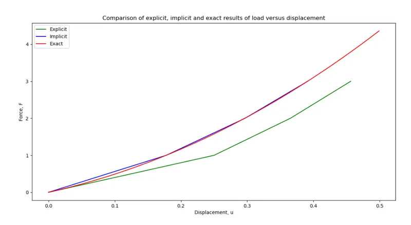
It is evident from the plot that the explicit analysis drifts from the exact solution.

The drift from the exact solution illustrates the lack of equilibrium between the internal and external forces. To correct this problem an implicit analysis is required.

The Newton-Raphson iterations correct the incremental steps so that they land on the exact solution according to the specified tolerance. Excellent agreement is achieved with just 3 increments and in each step, only two Newton-Raphson iterations are required.

DISCUSSION:

As per the above steps, we can use both implicit and explicit solvers to solve the same type of problems. The only difference is an approach to time increment.

The implicit analysis allows you to select how big the time increment should be, this increment will take some time to compute since it has to iterate for global equilibrium first. But we can make it reasonably big for our analysis.

Explicit time increments calculate really fast because they don't iterate the global equilibrium, but the time increment there is not the user's choice. Solver simply assumes an acceptable time increment and goes with it.

The speed of computing is exactly the difference between implicit and explicit. of course, the size of the explicit step depends on our model, and computing times depend on the system hardware.

The debate on what type of solver is better depends on the type of problem and accuracy we need.