Week - 2 - Explicit and Implicit Analysis

• Aim: To explain the difference betweeen implicit and explicit method used in FEM and solve the given equation using both implicit and explicit method and plot and compare the results.

Explicit and Implicit solvers are used to solve non linear transient dynamic problems, in which the load applied is very fast. In such cases, the time is incremented, not the load. Explicit and Implicit analysis divide the time into smaller increments to analyse the problem. Implicit and Explicit analysis differ in the approach to time incrementation. In Implicit analysis each time increment has to converge, and the time increments can be very large. Explicit on the other hand doesn’t have to converge each increment, but for the solution to be accurate time increments must be super small.

Implicit: In Implicit analysis, global equilibrium is established for each time increment, i.e each increment has to converge. Convergence is achieved after every time timestep by incorporating correction scheme to minimize the residual. The finite element variables are calculated after the global equilibrium is established. The time increments can be very big, since global equilibrium is verified at each time increment. This results in high computational time, since more iterations are needed for getting global equilibrium. Implicit method can be used for slow analysis, which are happening for several seconds.

Explicit: In explicit analysis, no convergence for each step is needed. There are no iterations to be done. The local finite element variables are calculated without verifying global equilibrium. Therefore, calculations are extremely fast in explicit analysis. However, the time steps should be extremely small. It is conditionally stable method.

• Solving the given equation F(u) = u³+9u²+4u using both Explicit and Implicit methods ( Tolerence of 0.01 is used).

Calculations by explicit method:

Let ∆F = 1 (incremental externally applied force), ∆u = incremental displacement,  u = displacement, f = internal force and F = external force and k = stiffness. No. of load increments = 3

k = Stiffness = 3u² + 18u +4.

Step 1: First load increment, ∆F =1

u₀ = 0, k(u₀) = 3(u₀)² + 18u₀ +4 = (3x0²) + (18x0) + 4 = 4

∆u₁ = ∆F/k(u₀) = 1/4 = 0.25

u₁ = u₀ + ∆u₁  = 0 + 0.25 = 0.25

Step 2 : Second load increment, ∆F =1

u₁ = 0.25, k(u₁) = 3(u₁)² + 18u₁ + 4 = (3x0.25²) + (18x0.25) + 4 = 8.6875

∆u₂ = ∆F/k(u₁) = 1/8.6875 = 0.115

u₂ = u₁ + ∆u₂  = 0.25 + 0.115 = 0.365

Step 3: Third load increment, ∆F =1

u₂ = 0.365, k(u₂) = 3(u₂)² + 18u₂ +4 = (3x0.365²) + (18x0.365) + 4 = 10.972

∆u₃ =  ∆F/k(u₂) = 1/10.972 = 0.091

u₃ = u₂ + ∆u₃  = 0.365 + 0.091 = 0.456

From the above three steps, the following results are obtained:

F_ext  =  ∆F+ ∆F + ∆F = 3.0;

F_int  = (u₃)³ + 9(u₃)²  + 4u₃ = (0.456)³ + 9(0.456)²  + 4(0.456) = 3.790

From the results, it is observed that F_ext ≠ F_int. The external and internal forces are not in equilibrium. Summary of the results from the explicit analysis are shown in the table below:

Step i	∆Fi	∆ui	ui	(Fext)i	(Fint)i	R = Fint  - Fext
1	1	0.25	0.25	1	1.578	0.578
2	1	0.115	0.365	2	2.709	0.709
3	1	0.091	0.456	3	3.790	0.790

Calculations by implicit method:

Given tolerance for the residual R is 0.01 i.e R < 10^-2

Step 1: Second load increment, ∆F = 1

u₀ = 0, k(u₀) = 3(u₀)² + 18u₀ +4 = (3x0²) + (18x0) + 4 = 4

∆u₁ =  ∆F/k(u₀) = 1/4 = 0.25

u₁ = u₀ + ∆u₁  = 0 + 0.25 = 0.25

f(u₁) = (u₁)³ + 9(u₁)² + 4u₁ = (0.25)³  + 9(0.25)² + 4(0.25) = 1.578       

Residual, R⁰ = f₁ - ∆F₁ = 1.5781 – 1 = 0.578

R⁰  > 0.01

Newton – Raphson iterations are necessary to obtain correction so that residual is achieved within tolerance value.

u₁⁽⁰⁾  = 0.25

k(u₁⁽⁰⁾) = (3x0.25²) + (18x0.25) + 4 = 8.6875

δu¹ = -[k(u₁⁽⁰⁾)]^-1 R⁰ = -[8.6875]^-1 . 0.578 = -0.06653

The updated value of u₁⁽¹⁾ = u₀ + δu¹ = 0.25 + (-0.06653) = 0.1835

Check the residual again,

F_ext = 1

f_int = (u₁¹)³ + 9(u₁¹)²  +  4(u₁¹) = 0.1835³ + 9(0.1835)² + 4(0.1835) = 1.0432

R¹ = f_int - F_ext  = 1.0432 - 1 = 0.0432

R¹ > 10^-2 , therefore another Newton Raphson iteration is necessary.

Second iteration:

k(u₁⁽¹⁾) = (3x0.1835²) + (18x0.1835) + 4 = 7.4040

δu² = δu¹-[k(u₁⁽¹⁾)]^-1 R¹ = -0.06653-[7.4040]^-1 . 0.039 = -0.0723

u₁⁽²⁾ = u₁ + δu² = 0.25 + (-0.0718) = 0.1777

f_int = (u₂¹)³ + 9(u₁²)²  +  4(u₁²) = 0.1777³ + 9(0.1777)² + 4 (0.1777) = 1.0006

R² = f_int - F_ext  = 1.0006-1 = 0.0006

No further iterations are required, since residual is within the tolerance.

Final value of u₁ = 0.1777

Step 2: Second load increment, ∆F = 1

u₁ = 0.1777, k(u₁) = (3x0.1777²) + (18x0.1777) + 4 = 7.2933

∆u₂ =  ∆F/k(u₁) = 1/7.2933 = 0.1371

u₂ = u₁ + ∆u₂ = 0.1777 + 0.1371 = 0.3148

f(u₂) = (u₂)³ + 9(u₂)² + 4u₂ = (0.3148)³  + 9(0.3148)² + 4(0.3148) = 2.1823      

Residual, R⁰ = f _int- F_ext = 2.1823 – 2 = 0.1823

R⁰  > 0.01

Newton – Raphson iterations are necessary to obtain correction so that residual is achieved within tolerance value.

k(u₂⁽⁰⁾) = (3x0.3148²) + (18x0.3148) + 4 = 9.9637

δu¹ = -[k(u₂⁽⁰⁾)]^-1 R⁰ = -[9.9637]^-1 . 0.1823 = -0.0183

The updated value of u₂⁽¹⁾ = u₂⁽⁰⁾ + δu¹ = 0.3148 + (-0.0.183) = 0.2965

Check the residual again,

f_int = (u₂¹)³ + 9(u₂¹)²  +  4(u₂¹) = 0.2965³ + 9(0.2965)² + 4(0.2965) = 2.003

R¹ = f_int - F_ext  = 2.003 - 2 =  0.003

No further iterations are required, since residual is within the tolerance.

Final value of u₂ = 0.2965

Step 3: Third load increment, ∆F = 1

k(u₂) = (3x0.2965²) + (18x0.2965) + 4 = 9.6007

∆u₃ =  ∆F/k(u₂) = 1/9.6007 = 0.1041

U₃ = u₂ + ∆u₃ = 0.2965 + 0.1041 = 0.4006

f(u₃) = (u₃)³ + 9(u₃)² + 4u₃ = (0.4006)³  + 9(0.4006)² + 4(0.4006) = 3.111      

Residual, R⁰ = f _int- F_ext = 3.111 – 3 = 0.111

R⁰  > 10^-2

Newton – Raphson iterations are necessary to obtain correction so that residual is achieved within tolerance value.

k(u₃⁽⁰⁾) = (3x0.4006²) + (18x0.4006) + 4 = 11.6922

δu¹ = -[k(u₃⁽⁰⁾)]^-1 R⁰ = -[11.6922]^-1 . 0.111 = -0.0094

u₃⁽¹⁾ = u₃ + δu¹ = 0.4006 + (-0.0094) = 0.3911

f_int = (u₃¹)³ + 9(u₃¹)²  +  4(u₃¹) = 0.3911³ + 9(0.3911)² + 4 (0.3911) = 3.0008

R¹ = f_int - F_ext  = 3.0008 - 3 = 0.0008

No further iterations are required, since residual is within the tolerance.

Final value of u₃ = 0.3911

Summary of implicit analysis:

Step i	∆Fi	ui	Fext	fint	fint - Fext = R
1	1	0.1777	1	1.006	0.004
2	1	0.2965	2	2.003	0.003
3	1	0.3911	3	3.0008	0.0008

• Results plot:

Result plot for the exact solution and solution obtained by implicit and explicit method is shown below.

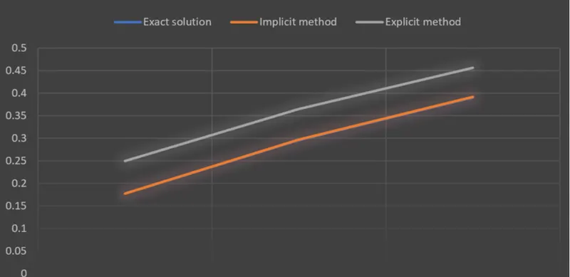
It can be seen from the graph that the plot of exact solution and solution obtained by implicit method are almost identical. On the other hand, the solution obtained by explicit method drifts away from the exact solution, although the no. of increments are increased. The drift of solution from exact solution indicates lack of equilibrium between internal and external forces. The Newton Raphson iterations used in implicit method correct the incremental steps, so that obtained results are close to true solution. But the selection of the method to be used for analysis is mostly dependend on the type of analysis to be performed.

• Conclusion: Thus, the difference between the implicit and explicit method is discussed and explained by solving the given example and the results are plotted and compared.