Week - 2 - Explicit and Implicit Analysis

Both implicit and explicit methods are dedicated to solve dynamic events which has incremental loads.

The dynamic governing equation can be given by

[M] {x’’} + [C] {x’} + [K] {x} = {f}

the forces may be time dependent or may be constant.

Where,

M= mass matrix

C = Damping matrix

K = stiffness matrix

X’’ = acceleration

X’= velocity

X = displacement

Implicit analysis

• Implicit analysis is generally used for static and time independent problems in other words for equilibrium problems only where sum of all forces are zero.
• In implicit analysis the solution is obtained by solving an equation that includes both current later stages of the system so that at each time the increment has to be converged using iterative method.
• We cannot discriminate the mathematical equation in implicit analysis. In implicit we solve for {x} which is displacement by inversing the stiffness matrix then the governing equation will be

[M] {x’’} + [C] {x’} + [K] {x} = {f}

[K] {x} = {f} – ([M] {x’’} + [C] {x’})

{x} = `[K]^-1` ({f} – ([M] {x’’} + [C] {x’}))

For static analysis the mass matrix [M] and damping matrix [C] is zero so the equation becomes

{x} = `[K]^-1`{f}

• We can use the implicit analysis to solve dynamic and nonlinear problems but the inversion of the stiffness matrix is complicated and time consuming and at every interval the solution must converge so this makes the analysis significantly slower but the implicit analysis is un conditionally stable and the sum of the all the forces in implicit analysis are zero
• The effect of strain rate and solver events are negligible (below 10 units/sec)
• The time step and increment in the implicit analysis is large when it’s compared to explicit.

Explicit analysis

• The explicit analysis is preferred for nonlinear and dynamic problems where time variable is the associated with the problem. Explicit analysis is used to calculate state of the given system at different time from the current time.
• We can discriminate the mathematical equation in explicit analysis. In explicit we solve for {x’’} which is acceleration by inversing the mass matrix then the governing equation will be

[M] {x’’} + [C] {x’} + [K] {x} = {f}

[M] {x’’} = {f} – ([C] {x’} + [K] {x})

{x’’} = [M]^-1 ({f} – ([C] {x’} + [K] {x}))

• Here mass matrix is lumped and diagonal matrix thus inversion of diagonal matrix is simple and computation is much faster but the analysis may not be stable.
• In implicit there is no need of iterating the solution at each increment and the time taken by the explicit analysis is depends on the wave propagation speed and characteristic length of the element.
• Explicit analysis is very handy when the strain rates and velocities are above 10 units / sec and sum of all the forces are equal to the product of mass and acceleration. I;e (F = ma)
• Since the time step is very small and the computation speed will be higher than that of the implicit.

Aim:

The objective of this project is to calculate and solve the given equation in Explicit and Implicit method and to comapare the output values (displacement values) of both the methods by plotting graph.

Procedure and Calculations:

Explicit Analysis

`F(u)` =`u^3+9u^2+4u` --------------------------------------- 1.

`K(u)`= `f(u)` / `d(u)` = `3u^2+18u+4` --------------------2.

Step- 1

`u0`= 0

`k(uo)` = 3x `0^2`+ 18x0 +4 = 4

∆F = 1

∆u1 = ∆F / `k(u0)` = 1/4 = 0.25

`u1 = u0 + ∆u1`= 0 +0.25 = 0.25

Step- 2

u1 = 0.25 , ∆F = 1

`k(u1)` = 3x`0.25^2` + 18x0.25 + 4 = 8.6875

`∆u2` = ∆F /`k(u1)` = 1/8.6875 = 0.1151

`u2 = u1 + ∆u2` = 0.25 + 0.1151 = 0.3651

Step- 3

`u2` = 0.3651 , ∆F = 1

`k(u2)` = 3x`0.3651^2` + 18x0.3651 + 4 = 10.9717

`∆u3` = ∆F / `k(u2)` = 1/10.9717 = 0.0911

`u3 = u2 + ∆u3` = 0.3651 + 0.0911 = 0.4562`0.4562^2`

`F ext`= ∆F + ∆F + ∆F = 1 + 1 + 1 = 3

f int = F(u) = `u^3+9u^2+4u`

`f(u1)` = `0.25^3` + 9 x `0.25^2` + 4 x 0.25 = 1.5781

`f(u2)` = `0.3651^3`+ 9 x`0.3651^2` + 4 x 0.3651 = 2.7087

`f(u3)` = 0.4562^3 + 9 x0.4562^2 + 4 x 0.4562 = 3.7928

R = F int - f ext

R1 = 1.5781 – 1 = 0.5781

R2 = 2.7087 – 2 = 0.7087

R3 = 3.7928 – 3 = 0.7928

Summary of explicit method

Step (i)	∆F(i)	∆u(i)	Ui	F ext	f int	R = f int - F ext
1	1	0.25	0.25	1	1.5781	0.5781
2	1	0.1151	0.3651	2	2.7087	0.7087
3	1	0.0911	0.4562	3	3.7928	0.7928

Implicit Analysis

Tolerance value = 0.001

Step – 1

u0= 0, ∆F = 1, `k(u0)` = 4, = 1.5781, `u1= u0+ ∆u1` = 0 +0.25 = 0.25

`u1` = ∆F / `k(u0)` = 1/4 = 0.25

`k(u1)` = 3x`0.25^2`+ 18x0.25 + 4 = 8.6875 checking residual

R0 = 1.5781 – 1 = 0.5781

║R0 ║> `10^-3`

Correction to `u1 = u1_0` using Newton – Raphson iteration

`δu^1 = - 〖[ k (u_1^((0)))] 〗^(-1) R^((0))` = - 1/ 8.6875 x 0.5781 = - 0.0665

Updated value of `u1_1 = u1_0`+ `delta`u1` = 0.25 – 0.0665 = 0.1835

Checking residual again F ext = 1

f ext = `F(u) = u^3+9u^2+4u` where u = u1_1

= `0.1835^3`+ 9 x `0.1835^2`+ 4 x 0.1835 = 1.0432

R1 =f int - F ext = 1.0432 – 1 = 0.0432

║R1║>`10^-3`

New total correction to u1 = u1_0 using Newton – Raphson iteration

`δu^2 = δu^1 - 〖 [ k (u_1^((1)))] 〗^(-1) R^((0))`

= - 0.0665 – 1 / 7.4040 x 0.0432 = - 0.0723

Updated value of `u1_2`= `u1_0` + `delta`u2` = 0.25 – 0`0.1777^2`.0723 = 0.1777

Checking residual again F ext = 1

f int = `F(u) = u^3+9u^2+4u`where `u = u1_2` = 1.0006

R2 = f int - F ext = 1.0006 – 1 = 0.0006

║R2║ < No further iteration

`therefore` The final value is `u1 = u1_2` = 0.1777

Step – 2

`u1 =` 0.1777 , ∆F = 1

`k(u1)` = 3x 0.1777^2 + 18x0.1777 + 4 = 7.2933

∆u2 = ∆F / `k(u1)`= 1/7.2933 = 0.1371

`u2 = u1 + ∆u2` = 0.1777 + 0.1371 = 0.3148 checking residual

f int =`F(u) = u^3+9u^2+4u` where `u = u2`

= 2.1823

R0 = 2.1823 – 2 = 0.1823

║R0║> `10^-3`

Correction to `u0 = u0_2` using Newton – Raphson iteration

`δu^1 = - 〖[ k (u_2^((0)))] 〗^(-1) R^((0))` = - 1/ 9.9637 x 0.1823 = - 0.0183

Updated value of `u1_2 = u0_2` + `delta u1` = 0.3148 – 0.0183 = 0.2965

Checking residual again F ext = 1

f int = `F(u) = u^3+9u^2+4u` where`u =u1_2`

= `0.2965^3`+ 9 x `0.2965^2` + 4 x 0.2965 = 2.0033

R1 = f int - F ext = 2.0033 – 2 = 0.0033

║R1║> `10^-3`

New total correction to `u1= u1_0` using Newton – Raphson iteration

`δu^2 = δu^1 - 〖 [ k (u_2^((1)))] 〗^(-1) R^((0))`

= - 0.0183 – 1 / 9.6007 x 0.0033 = - 0.0186

Updated value of `u2_2 = u2_0`+ `deltau2` = 0.3148 – 0.0186 = 0.2962

Checking residual again F ext = 1

f int = `F(u) = u^3+9u^2+4u` where `u =u2_2`

R2 = f int - F ext = 2.00039 – 2 = 0.00039

║R2║`< 10^-3`

`therefore`The final value is`u2 = u2_2`= 0.2962

Step – 3

`u2 = 0.2962` , ∆F = 1

`k(u2)`= 3x`0.2962^2` + 18x0.2962 + 4 = 9.5948

∆u3 = ∆F /`ku(2)` = 1/9.5948 = 0.1042

`u3= u2 + ∆u3` = 0.2962 + 0.1042 = 0.4004 checking residual

f int =`F(u) = u^3+9u^2+4u` where`u =u3`

= 3.1087

R0 = 3.1087 – 3 = 0.1087

║R0║>`10^-3`

Correction to `u3 = u3_0` using Newton – Raphson iteration

`δu^1 = - 〖[ k (u_3^((0)))] 〗^(-1) R^((0))`

= - 1/ 11.6882 x 0.1087 = - 0.0093

Updated value of `u3_1 = u3_0`+ `deltau1` = 0.4004 – 0.0093 = 0.3911

Checking residual again F ext = 1

f int =`F(u) = u^3+9u^2+4u` where `u =u3_1`

= 0.3911^3 + 9 x 0.3911^2 + 4 x 0.3911 = 3.00085

R1 = f int - F ext = 3.00085 – 3 = 0.00085

║R1║<`10^-3`

`therefore` The final value is `u3 = u3_1` = 0.3911

Summary of Implicit analysis

Step (i)	∆F(i)	ui	F ext	f int	R = f int - F ext
1	1	0.1777	1	1.00060	0.00060
2	1	0.2962	2	2.00039	0.00039
3	1	0.3911	3	3.00085	0.00085

Results:

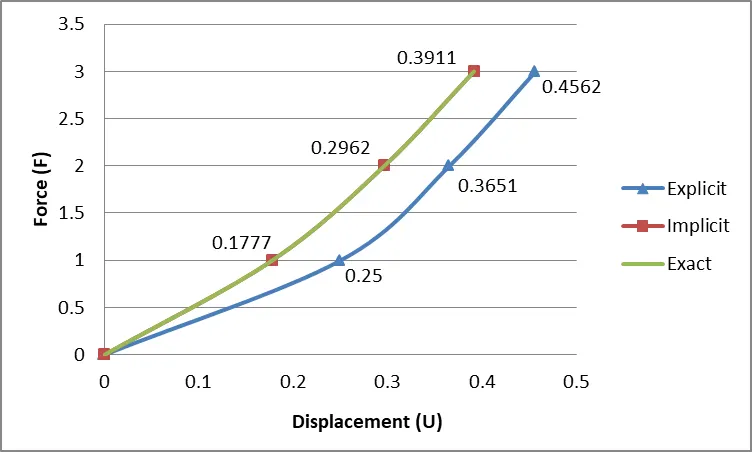
Conclusion:

The given equation is solved using both implict and explicit approch, as the result graph indicates the implicit approch converges the values to the exact results but requires lot of iterations thus makes it computationally time consuming where as the explict approch gives the less accurate results but the solution time is much faster than the implicit approch.