Week - 2 - Explicit and Implicit Analysis
AIM:
-
Introduction to Explicit Methods:
The explicit method allows solving problems element by element. Compared with the implicit method, it does not require the general matrix, since the velocity and displacement nodes can be counted directly, using the central difference integration scheme. However, the time step is limited by the size of the numerical stability. Accordingly, this method is considered as conditionally stable, because if the time step is too large, there will be a significant numerical error. In this method, there is no requirement for balance, so it is suitable for highly dynamic analysis, such as high velocity impact.
- Explicit finite element codes are now used extensively in aerospace, nuclear, and rail technology. In this way, bird strike, safety of transport bottles, train crash, etc., can be simulated. The best-known commercial software analyses for the explicit method are: PAM-CRASH, LS-DYNA, and RADIOSS.
- When we apply an explicit time discretization scheme, obviously considering the nodes in the computational domain, the variables at time step n+1 simply depend only on the known values at the time step n. However, stability can be a problem in the case of an explicit time discretization method. A numerical scheme is stable if errors do not grow from one time step to the next time step.
Introduction to Implicit Methods:
In the implicit method, general equilibrium is achieved by iteration at first, followed by evaluation of local element variables. If the balance is not achieved, this method becomes expensive for calculation, since the matrix coefficients should recalculate with different time steps. The implicit method is unconditionally stable, allowing the use of larger increment time steps. It is suitable for problems that tend to be highly linear, static, and quasi-static.
- Commercially available software for the application of implicit methods are: ABAQUS, ANSYS, and NASTRAN.
- In implicit method, the variables at the time n+1 can depend on both values at time n and n+1. Therefore, an implicit method can be classified into semi-implicit or fully implicit schemes, where the variables at the time n+1 depend on both values at the time steps n and n+1, or only time step n+1, respectively.
- Thus, in both schemes of an implicit method, a system of equations must be solved, which is not the case for the explicit method. For the case of highly nonlinear equations, when all the 3D governing equations are solved simultaneously, a huge storage space might be required. However, it should be noted that a fully implicit method is unconditionally stable.
Analysis:
Here we will solve the equation using Explicit and Implicit methods and compare the results.
Equation to solve is given as below:
`f(u)=u^3+9u^2+4u`
Tolerance: 10 -2
Procedure:
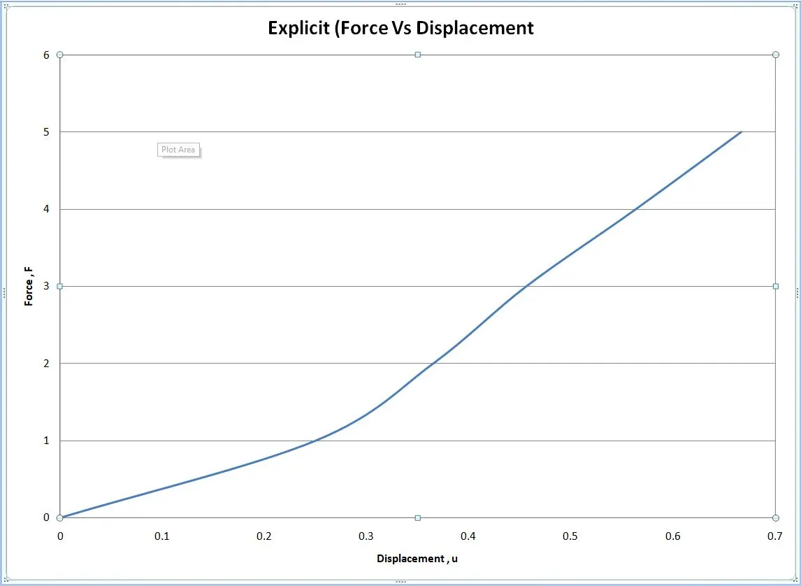
Explicit Method:
- If the nonlinear force versus displacement relationship is not known, but the stiffness is known, it is possible to construct the graph of force versus displacement numerically.
- It can be done by using an incremental explicit load control scheme.
`f(u)=u^3+9u^2+4u`
Above equation can be solved using Explicit method as follows:
Now, F = k* x , where k is the Stiffness.
- To get the Stiffness, differentiate it with respect to displacement
`f(u)=u^3+9u^2+4u`
`k(u) = (dF)/(du) = 3u^2 + 18u + 4`
- Now we will use three equal incremental load steps of external force to give loading of `∆F = 1.`
Variables are as given below:
- U = Displacement
- F =External Force
- F = Internal Force
- k =Stiffness
- `∆u`= Incremental Displacement
- `∆F`= Incremental externally applied force
Here, Relationship `∆F` = k `∆u` is used for finding Incremental Displacements.
The Analysis proceeds as follows:
Step_1:
`uo`= 0.0,
`k(uo) = 3(0)2 + 18(0) + 4 = 4`
`∆F = 1`
`∆u1` =`∆F`/ `k(uo)`= 1 / 4 = 0.25,`
`u1 `= `u0` +` ∆u1` = 0 + 1 / 4 = 0.25
FExternal = `∆F `= 1
FInternal = `u1^3+9u1^2+4u1` = (0.25)^3+9(0.25)^2+4(0.25)` = 1.5781
R = FInternal - FExternal = 1.5781 – 1 = 0.5781
Step_2:
`u1`= 0.25,
`k(u1) = 3(0.25)2 + 18(0.25) + 4 = 8.6875``
`∆F = 1`
`∆u2 `= `∆F`/ `k(u1)`= 1 / 8.6875 = 0.115107,
`u2` = `u1` +` ∆u2` = 0.25 + 8.6875 = 0.3651
FExternal =`∆F`+`∆F` = 1+1= 2
FInternal = `u2^3+9u2^2+4u2` = (0.3651)^3+9(0.3651)^2+4(0.3651)` = 2.70874
R = FInternal - FExternal = 2.70874 – 2 = 0.70874
Step_3:
`u2`= 0.3651,
`k(u1) = 3(0.365)2 + 18(0.3651) + 4 = 10.97139``
`∆F = 1`
`∆u3 `= `∆F`/ `k(u1)`= 1 / 10.97139 = 0.091146,
`u3` = `u2` +` ∆u3` = 0.3651 + 0.091146 = 0.4562
FExternal =`∆F`+`∆F` +`∆F`= 1+1+1 = 3
FInternal = `u3^3+9u3^2+4u3` = (0.4562)^3+9(0.4562)^2+4(0.4562)` = 3.7928
R = FInternal - FExternal = 3.7928 – 3 = 0.7928
Summary of the main results for the explicit analysis detailed as given below:

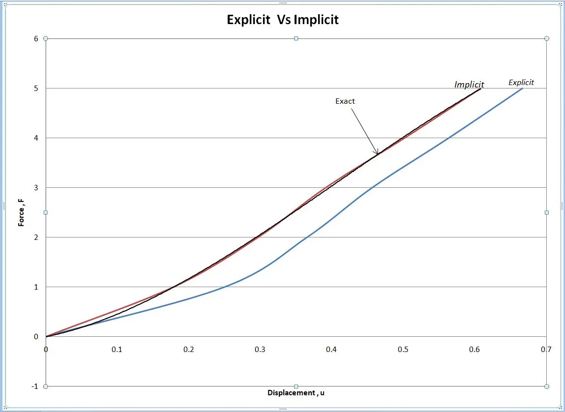
It is evident from the results that external and internal forces are NOT in equilibrium because
`Funderset(External)!= ``Funderset(Internal)`Implicit Method:
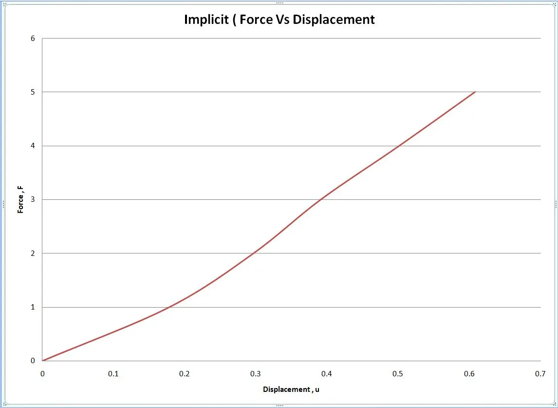
An implicit analysis is the same as the explicit analysis, except that at the end of each step Newton-Raphson iterations are used to enforce equilibrium before moving to the next step. Basically, an incremental force is applied to advance the solution forward at the beginning of a step. However, internal forces and external forces will not be in equilibrium unless the stiffness is linear for the given step. Hence, in order to achieve equilibrium, corrections must be made to the displacement. This is accomplished by using Newton-Raphson iterations to minimize the residual, `R(u) = Fint − Fext`.
Expanding the residual as a Taylor series about the current displacement `uoversetj` gives,
R(j+1)= `Roversetj` `uoversetj` ``dR(`uoversetj`)/du```(delta uoverset(j+1`)``+......= `Roversetj`+ k `uoversetj``(delta uoverset(j+1`)+.....
By neglecting higher order terms in the series, setting
`Roverset(j+1`=0 and solving for `(delta uoverset(j+1`)
the following correction is obtained:
`(delta uoverset(j+1`) = -[k(`uoversetj`)]`overset(-1)` `Roversetj`
Notice that the iteration variable is j and it may take several iterations for the norm of the residual, `||R||`, to be reduced below the chosen tolerance criteria.
Here, we have tolerance criteria is of `10overset(-2)`.
The Analysis proceeds as follows:
Step_1:
`uo`= 0.0,
`k(uo) = 3(0)2 + 18(0) + 4 = 4`
`∆F = 1`
`∆u1` =`∆F`/ `k(uo)`= 1 / 4 = 0.25,`
`u1 `= `u0` +` ∆u1` = 0 + 1 / 4 = 0.25
FExternal = `∆F `= 1
FInternal = `u1^3+9u1^2+4u1` = (0.25)^3+9(0.25)^2+4(0.25)` = 1.5781
Checking Residuals:
R = FInternal - FExternal = 1.5781 – 1 = 0.5781
||R|| = 10^(-2)
So, Newton-Raphson iterations are necessary.
Calculate the correction to u1 = u1^(0)
k u1 = 8.6875 & R(0)=0.578152
`delta uoverset(1)` =` -[k * u1overset((0))`]`overset(-1) ` `Roverset((0))```
= `-[(8.6875)]overset(-1` (0.578152)
`delta uoverset(1)`= -0.0665467
Now, updating the value,
`u1overset((1)) ` =` u1overset((0)) ``+delta uoverset((1))`
`nbsp; = 0.25 + (-0.06654)`
`u1overset((1)) ` = 0.18346
Now, checking Residuals,
Fext = `∆F = 1`
Fint = `(u1overset((1)``)^3 + 9(u1overset((1)``)^2 + 4u1overset((1)```
= `(0.18346)^3 +9(0.18346)^2 + 4 (0.18346)`
Fint = 1.03736
Now, `Roverset((1)``` = F Internal - F External = 1.03736 - 1 = 0.03736
``||`Roverset(1)`||`` `gt` `10overset(-2)`
So, Newton-Raphson iterations are necessary.
So, k(u1) = `3u1overset(2)` + `18u1 +4`
= `3(0.18346)^2 +18(0.18346) + 4`
k(u1) = 7.4032527
So, calculating new total correction to `u1 = u1overset((0)`
`delta u overset((2)) ` =`delta u overset((1) ``- [k (u1)overset((1))``]overset(-1)` `Roverset((1))`
= -0.066547-`[7.40325]^(-1) (0.03736)
δ u^(2) = 0.071593``
Now, updating the value,
`u1^(2) = u1+δ uo^(2))
= 0.25 + (-0.071593)
`u1^(2)= 0.178407`
Now, checking Residuals,
Fext = `∆F = 1`
Fint = u1^(2)^3 + 9(u1^(2)^2 + 4u^(2)
= `(0.178407)^3 +9(0.178407)^2 + 4 (0.178407)`
Fint = 1.005767
Now, `Ro^(2) = F Internal - F External = 1.055767 - 1 = 0.005767
||Ro|| = 10^(-2)
So, Newton-Raphson iterations are not necessary.
So, Final value is u1 = `u1overset((2))` = 0.178407
Step_2:
`u1`= 0.178407,
`k(u1) = 3(0.178407)2 + 18(0.178407) + 4 = 7.306813`
`∆F = 1`
`∆u2` =`∆F`/ `k(u1)`= 1 / 7.306813= 0.136858`
`u2 `= `u1` +` ∆u2` = 0.178407 + 0.136858 = 0.31526
FExternal = `∆F `+`∆F `= 1 +1 = 2
FInternal = `u2^3+9u2^2+4u2` = (0.31526)^3+9(0.31526)^2+4(0.31526)` = 2.186873
Checking Residuals:
R = FInternal - FExternal = 2.186873 – 2 = 0.186873
||R(0)||=10^(-2)`
So, Newton-Raphson iterations are necessary.
So, k(u2) = `3u1^(2)` + `18u1 +4`
= `3(0.31526)^2 +18(0.31526) + 4`
k(u1) = 9.97278
So, calculating new total correction to `u1 = u1^0
δu(1) = - [k (u2)]^(-1) R((0))`
= -`[9.97278]^(-1) (0.186873)`
δu = 0.01873``
Now, updating the value,
= 0.31526 + (-0.01873)``
`u2^9(1) = 0.29653
Now, checking Residuals,
Fext = `∆F `+`∆F `= 1+1=2
Fint = `(u2)^3 + 9(u2)^2 + 4u2^1
= `(0.29653)^3 +9(0.29653)^2 + 4 (0.29653)`
Fint = 2.003563
Now, R(1)= F Internal - F External = 2.003563 - 2 = 0.003563
||R(1)|| = 10^(-2)`
So, Newton-Raphson iterations are not necessary.
So, Final value is u2 = `u2overset((1))` = 0.29653
Step_3:
`u2`= 0.29653,
`k(u2) = 3(0.29653)2 + 18(0.29653) + 4 = 9.60133`
`∆F = 1`
`∆u3` =`∆F`/ `k(u2)`= 1 / 9.60133= 0.104152`
`u3 `= `u2` +` ∆u3` = 0.29653 + 0.104152 = 0.40068
FExternal = `∆F `+`∆F `+`∆F `= 1 +1+1 = 3
FInternal = `u3^3+9u3^2+4u3` = (0.40068)^3+9(0.40068)^2+4(0.40068)` = 3.11194
Checking Residuals:
R = FInternal - FExternal = 3.11194 – 3 = 0.11194
||R0||>10^-2
So, Newton-Raphson iterations are necessary.
So, k(u3) = `3u3^2 + 18u3 +4
= `3(0.40068)^2 +18(0.40068) + 4`
k(u3) = 11.6938
So, calculating new total correction to `u2 = u2^0
δu^2= -[k(u3)^0]^-1 R^0
= -`[11.6938]^(-1)(0.11194)`
δu^2 = -0.009572``
Now, updating the value,
`u3overset((1)) ` =` u3overset((0)) ``+delta uoverset((2))`
= 0.40068 + (-0.009572)``
`u3overset((1)) `` = 0.391108`
Now, checking Residuals,
Fext = `∆F `+`∆F `+`∆F `= 1+1+1=3
Fint = (u3o(1)^3 + 9(u3(1)^2 + 4u3(1)```
= `(0.391108)^3 +9(0.391108)^2 + 4 (0.391108)`
Fint = 3.000941
Now, `Roverset((1)``` = F Internal - F External = 3.000941 - 3 = 0.000941
``||`Roverset(1)`||`` `lt` `10overset(-2)`
So, Newton-Raphson iterations are not necessary.
So, Final value is u3 = u3(1) = 0.391108
Summary of the main results for the explicit analysis detailed as given below:

It is evident from the results that external and internal forces are coming into equilibrium because
`F(External)approx ``F(Internal)`Plots:
Explicit Method:
Implicit Method:
Comparison between Explicit and Implicit and Exact solution:
Discussion:
We already agreed that you can use both implicit and explicit solvers to solve the same type of problems. The only difference is in approach to time incrementation. But it is not a trivial thing! If the difference would be small, nobody would care to implement both.
Both implicit and explicit solvers have some areas where they shine. And there is an overlap in their use:
- The implicit analysis allows you to select how big the time increment should be! This increment will take some time to compute since it has to iterate for global equilibrium first. But you can make it “reasonably big” for your analysis.
- Explicit time increments calculate really fast! Simply because they do not iterate for global equilibrium… but the time increment there is not your choice! Solver simply assumes, that the “acceptable” time increment is “X” and goes with it. Note, that this “X” can easily be something like 5e-7s… This is super small! To solve a problem happening over 1s, you would need 2 000 000 increments!
- And that is it! The speed of computing is exactly the difference between implicit and explicit. Of course, the size of explicit step depends on your model and computing times depends on your hardware