Week - 2 - Explicit and Implicit Analysis
Objective:
For this challenge we have to solve a simple non-linear problem by using the both implicit and explicit methods.
Introduction:
Explicit Analysis
It is a method for calculating the status of some systems at a time other than the present. It can alternatively be stated that the dependent
variables can be directly computed using existing numbers.
In circumstances when there is a dynamic equilibrium, the explicit analysis yields a faster solution. The explicit method's main use is to solve for
acceleration. Computationally, the explicit method is quick and affordable. Each increment is determined in a split second. Accuracy is not upheld.
The timestep must be very minimal.
Implicit Analysis
Using matrix inversions, it is a method of solving to find the unknown. An implicit method is used when a dependent variable is calculated using a
set of equations and the final solution requires an iterative process or a matrix.
The use of implicit approaches to tackle dynamic and nonlinear problems takes a long time. The increments are large, and as a result, the process
is slow. When compared to explicit methods, accuracy is higher. The model's reactivity to time may be different from that of a real model. At the
same time, parameters are interdependent.
When the events are much slower and the effects of strain rates are minimal, the implicit method is used. Once the growth of stress as a function
of strain has been established, implicit methods can be used to analyse it. Because the implicit method cannot be applied to every type of
differential operator, the so-called operator splitting method, in which the differential operator is rewritten as the sum of two complementary
operators, is sometimes recommended. To demonstrate how this works, a simple qualitative model will be used.Let Q be a quantity whose value
Qn+1 we want to compute at time t=(n+1)it, in terms of its value at time t=ndt, i.e., Qn+1=Qn+dtS, where S is the rate of change in Q.
S would be assessed in terms of known quantities at the previous time step n in an explicit numerical technique. At the new time step n+1, an
implicit approach, on the other hand, would assess some or all of the terms in S in terms of unknown quantities. It is said to be an implicit
specification of the new n+1 values because new quantities appear on both the left and right sides of the Qequation. To compute the new numbers,
a matrix or iterative solution is usually utilised.
The speed of computing is exactly the difference between implicit and explicit methods.
Procedure:
The given force equation f(u) = u3 +9u2 +4u
Stifness Equation K = df/du
k = 3u^2 +18u +4 ________(1)
To solve the above equation we use the both explicit and implicit analysis to plot the difference between the force and displacement.
- Explicit Analysis
solving these equation with 3 equal load increment with F = 1
Step -1
U(0) = 0
k(u) = 4
ΔF = 1
By sub the above values in the given eq,we get
Δu1 = F/ k(u)
= 1/4
=0.25
u1 = U0+ U1 = 0+0.25 = 0.25
F1 = (0.25^3)+9(0.25^2)+4(0.25)
= 0.015625+0.5625+1
=1.578125
Step -2
u1 =0.25
Sub the given value in eq 1
K(u1)= 3(0.25^2)+9(0.25^2)+4
=8.6875
ΔF=1
ΔU2= F/ (u2)
= 1/8.6875
= 0.1151
U2 =Δu1+Δu2
= 0.25+0.1151
= 0.3651
F2 = (0.365^3)+9(0.365^2)+4(0.3+651)
= 2.708
Step - 3
U2 = 0.3651
Sub the given value in eq 1
k(u2) = 3(0.3651^2)+18(0.3651)+4
= 10.97
ΔF=1
Δu3 = F/k(u3)=1/10.97
= 0.09114
u3 =Δu2+Δu3
u3= 0.365+0.09114
=0.4562
F3= (0.4652^3)+9(0.4652^2)+4(0.4562)
=3.7792
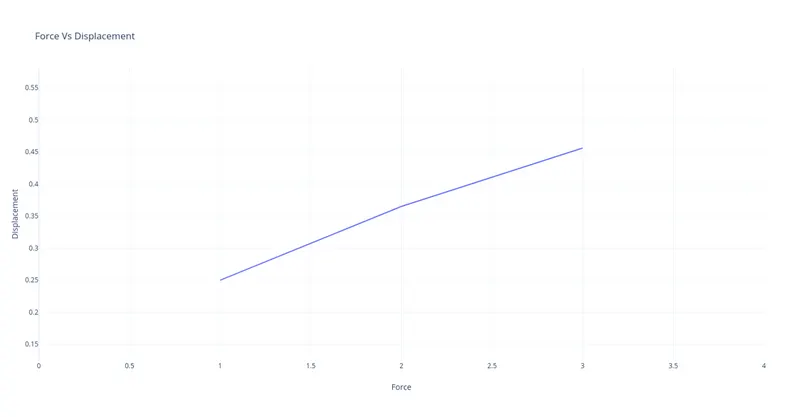
| Step | ΔF | U | F(EXT) | F(INT) | R=F(INT)-F(EXT) |
| 1 | 1 | 0.25 | 1 | 1.5781 | 0.5781 |
| 2 | 1 | 0.3651 | 2 | 2.7087 | 0.7087 |
| 3 | 1 | 0.4562 | 3 | 3.792 | 0.792 |
So from the table , it is noted that the difference in force i.e Residual is considerable , but the processing time is also very less.
- IMPLICIT ANALYSIS :
Step -1
U(0) = 0
K(u) = 4
ΔF =1
ΔU1 = F/`K(u) from k = df/du
= 1/4 = 0.25
F1 = (0.1834^3)+9(0.1834^2)+4(0.1834)
= 0.578125
R1 = F1(INT)=F1(EXT) = 0.578125
since R1> 0.01 newton raphson iteration are done.
NEWTON RAPHSON METHOD
It is a root finding algorithm which produces succesfully better approximation to the roots of a real valued function
I.e x1=x0-f(x0)/f1(x0)
By applying this we get
Δu1(1)=R1(1)/k(1U1(1)) = -0.066549
U1(2) = u1(1)+ U1(!)= 0.25-0.06654 =0.1834
F1(2) = 1.04249
R1(2) = 0.04249>0.01 so newton Raphson method is applied
ΔU1 (2) = R1(2)/K(u1(2))=0.07228
U1(3) = u1(2)+9(0.177^)+4(0.177)=1.00075
R1(3) = 0.000753
which is less than 0.01 so no need for Newton Raphson method
thus U1 =0.1772
F1 = 1.0007
R1=0.000753
Step -2
u1 = 0.1772
K(u) = 3(0.1772^2)+18(0.1772)+4 = 7.29
ΔF =1
ΔU2= F/K(u) = 0.137
u2 = U1+ u2 = 0.3148
F2 int = (0.177^3)+9(0.177^2)+4(0.177) = 2.182
R2 = F1int - F1et = 0.1822
since R2 > 0.01 Newton raphson method is done
Δu2(1) = R2(1)/K(u2(1)) = -0.018294
U2(2) = U2(1)+ u2(1)=0.3148-0.0182=0.2965
F2(2) = 2.0037
R2(2) = 0.00327<0.01 ;
so Newton raphson method is no further needed.
Thus,
U2 =0.2965
F2 = 2.0032
R2 = 0.00327
Step -3
U2 = 0.2965
K(u) = 3(0.2965^2) +18(0.2965)+4 = 9.60073
ΔF=1
Δu3 = F/k(u) = 0.1046
U3 = U2+ U3 = 0.4006
F3 int = (0.296^3)+9(0.2965^2)+4(0.2965)
R3 = F1int-F1ext = 0.111
It is greater than 0.01 so newton raphson method is done.
ΔU3 (1) = R3(1)/K(U3(1)) =-0.00949
U3 (2) = U3(1)+ U3(1)=0.3911
F3(@) = 3.0008
R3(2) = 0.00855<0.01
thus
u3 = 0.3911
F3 = 3.00855
R3 = 0.0085
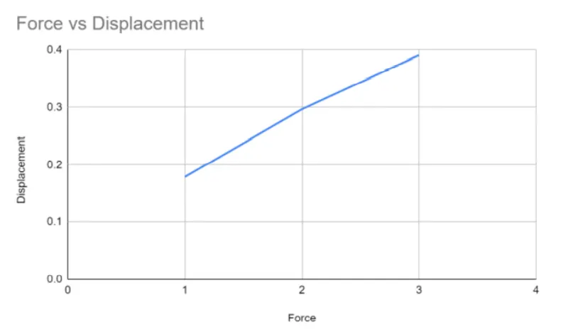
| Step | ΔF | U | F(EXT) | F(INT) | R=F(INT)-F(EXT) |
| 1 | 1 | 0.1772 | 1 | 1.0075 | 0.000753 |
| 2 | 1 | 0.965 | 2 | 2.003276 | 0.0032 |
| 3 | 1 | 0.3911 | 3 | 3.00855 | 0.0085 |
So from the table we can say that the Residual is very low and solution is accurate this is due to iteration performed by newton raphson method
But this Iteration Step has taken more time but this process is accurate and slow.
Conclusion:
The graph shows that implicit analysis is more accurate but takes longer and is solely dependent on element size and time steps, but
explicit analysis deviates somewhat from the exact result and requires more iteration to achieve a decent result.