Explicit and Implicit Analysis Theory part

AIM

To solve the given non linear equation by both implicit and explicit methods

Non-linear equation - F(u) = u3+9u2+4u

For the above equation force is the function of displacement.

Let us know about what is explicit and implicit analysis:

Explicit

Mass/inertia and damping are included, Dynamic analysis can be done via the explicit solver, No iteration is required as the nodal accelerations are solved directly, No inherent limit on the size of the time step, Time step must be less than the Courrant time step, Dose not require matrix inversion, Handles contact and material nonlinearities with relative ease, Once accelerations are known at time n, velocities are calculated at time n+1/2, and displacements at time n+1, from displacements comes strain, from strain comes stress & the cycle is repeated. The intent of this channel is to provide the complete solution for engineering problems related to Structural, Thermal & Fluid flow.

Explicit analyses aim to solve for acceleration (or otherwise {x´´}). In most cases, the mass matrix is considered as “lumped” and thus a diagonal matrix. Inversion of a diagonal matrix is straightforward and includes inversion of the terms on the diagonal only. Once the accelerations are calculated at the nth step, the velocity at n+1/2 step and displacement at n+1 step are calculated accordingly. In these calculations, the scheme is not unconditionally stable and thus smaller time steps are required. To be more precise, the time step in an explicit finite element analysis must be less than the courant time step (i.e., the time taken by a sound wave to travel across an element) while implicit analyses have no such limitations.

IMPLICIT

No effect of mass (inertia) or of damping, Static analysis is done using an implicit solver, solution of each step requires iterative solutions to establish equilibrium within a certain tolerance, Time steps are generally larger than explicit time steps, Requires a numerical solver to invert the stiffness matrix once or even several times over the course of a load/time step, which is expensive for large models.

One method of solving for the unknowns {x} is through matrix inversion (or equivalent processes). This is known as an implicit analysis. When the problem is nonlinear, the solution is obtained in a number of steps and the solution for the current step is based on the solution from the previous step. For large models, inverting the matrix is highly expensive and will require advanced iterative solvers (over standard direct solvers). Sometimes, this is also known as the backward Euler Intergration scheme. These solutions are unconditionally stable and facilitate larger time steps. Despite this advantage, the implicit methods can be extremely time-consuming when solving dynamic and nonlinear problems.

Time -dependent vs. Time - independent Analysis

For all nonlinear and non-static analyses, incremental load (also known as displacement steps) are needed. In more simplistic terminology, this means we need to break down the physics/time relationship to solve a mathematical problem. To do this, we form two groups: either time-dependent or time-independent problems. To solve these problems, we commonly use ‘implicit’ and/or ‘explicit’ methods.

We refer to problems as ‘time-dependent’ when the effects of acceleration are pronounced and cannot be neglected. For example, in a drop test, the highest force occurs within the first few milliseconds as the item decelerates to a halt. In this case, the effect of such a deceleration must be accounted for.

In contrast, when loads are slowly applied onto a structure or surface (i.e., when a monitor is placed onto a table) the loading can be considered ‘quasi-static’ or ‘time-independent’. This is because the loading time is slow enough that the acceleration effects are negligible.

IMPLICIT vs. EXPLICIT Problems

All of these problems are expressed through mathematical partial differential equations (PDE’s). While today’s computers can’t single-handedly solve PDE’s, they are equipped to solve matrix equations. These matrix equations can be linear or nonlinear. In most structural problems, the nonlinear equations fall into 3 categories:

• Material Nonlinearity: Where deformations and strains are large (i.e., polymer materials)
• Geometric Nonlinearity: Where strains are small, but rotations are large (i.e., thin structures)
• Boundary Nonlinearity: Due to non-linearity of boundary conditions, (i.e., contact problems)

In linear problems, the PDE’s reduce to a matrix equation as:

[K]{x} = {f}

and for non-linear static problems as:

[K(x)]{x} = {f}

For dynamic problems, the matrix equations come down to:

[M]{x´´} + [C]{x´} + [K]{x} = {f}

where (.‘) represents the derivative.

PROCEDURE AND SOLVING EQUATION

EXPLICIT METHOD

• If the non linear forces and displacement relationship is not known, but stiffness is defined, it is possible to plot the graph of force and displacement
• It is done by incremental load control

F(u) = u^3+9u^2+4u

stiffness,K(u) = dF(u)/du = 3u^2+18u+4

Displacement = Force/stiffness = F/K

Force increment = ΔF = 1

F = external force

f = internal force

STEP 1

u0 = 0.0

k(u0) = 3(0)^2+18(0)+4 = 4

ΔF = 1

Δu1 = ΔF/k(u0) = 1/4 = 0.25

u1 = u0+Δu1 = 0+1/4 = 0.25

F = ΔF = 1

f = u1^3+9u1^2+4u1 = (0.25)^3+9(0.25)^2+4(0.25) = 1.5781

Residual(R) = f - F = 1.5781-1 = 0.5781

STEP 2

u1 = 0.25

K(u1) = 3(0.25)^2+18(0.25)+4 = 8.6875

ΔF = 1

Δu2 = ΔF/K(u1) = 1/8.6875 = 0.1151

u2 = u1 + Δu2 = 0.25+0.1151 = 0.3651

F = ΔF+ΔF = 1+1 = 2

f = u2^3+9u2^2+4u2 = (0.3651)^3+9(0.3651)^2+4(0.3651) = 2.7087

Residual(R) = f - F = 2.7087 - 2 = 0.7087

STEP 3

u2 = 0.3651

K(u2) = 3(0.3651)^2+18(0.3651)+4 = 10.971

ΔF = 1

Δu3 = ΔF/K(u2) = 1/10.971 = 0.0911

u3 = u2+ Δu3 = 0.3651 + 0.0911 = 0.4562

F = ΔF+ΔF+ΔF = 1+1+1 = 3

f = (0.4562)^3+9(0.4562)^2+4(0.4562) = 3.7928

Residual(R) = f-F = 3.7928-3 = 0.7928

Summary of the explicit values:

STEP	ΔFi	Δui	ui	F(external)i	f(internal)i	R
1	1	0.25	0.25	1	1.5781	0.5781
2	1	0.1151	0.3651	2	2.7087	0.7087
3	1	0.0911	0.4562	3	3.7928	0.7928

Hence it is proved that forces are not in equilibrium in explicit method because

F(ext) ≠ f(int)

IMPLICIT METHOD

An implicit analysis is the same as the explicit analysis, except that at the end of each step
Newton-Raphson iterations are used to enforce equilibrium before moving to the next step.
Basically, an incremental force is applied to advance the solution forward at the beginning
of a step. However, internal forces and external forces will not be in equilibrium unless the
stiffness is linear for the given step. Hence, in order to achieve equilibrium, corrections must
be made to the displacement. This is accomplished by using Newton-Raphson iterations to
minimize the residual, R(u) = fint − Fext.

Expanding the residual as a Taylor series about the current displacement uj gives,

R^j+1 = R^j(u^j)+ dR(u^j)/du δu^j+1+... = R^j + K(u^j)δu^j+1.....

By neglecting higher order terms in the series, setting Rj+1 = 0 and solving for δu^j+1 the
following correction is obtained

δu^j+1 = -[k(u^j)]^-1R^j.

Notice that the iteration variable is j and it may take several iterations for the norm of the
residual, ∥R∥, to be reduced below the chosen tolerance criteria (for the example below a tolerance
of 10^−2 is chosen).

STEP 1

u0 = 0

k(u0) = 3(0)^2 + 18(0) + 4 = 4

ΔF = 1

Δu1 = ΔF/k(u0) = 1/4 = 0.25,

u1 = u0 + Δu1 = 0+1//4 = 0.25

F =ΔF = 1

f = u1^3+9u1^2 +4u1 = (0.25)^3 + 9(0.25)^2 + 4(0.25) = 1.5781

Residual (R) = f - F = 1.5781 - 1 = 0.5781

∥R^0∥ > 10^-2

So, Newton - Raphson iterations are necessary.

Calculate the correction to u1 = u1^(0)

k u1 = 8.6875 & R^0 = 0.5781

δu^1 = -[k.u1^(0)]^-1 R^(0)

= -[(8.6875)]^-1 (0.5781)

= -0.0665467

Now, updating the value,

u1^(1) = u1^(0) + δu^(-1)

= 0.25 + (- 0.06654)

u1^(1) = 0.18346

Residual (R)

F = ΔF = 1

f = (u1^(1))^3 + 9(u1(1))^2 + 4u1(1)

= (0.18346)^3 +9(0.18346)^2 + 4(0.18346)

= 1.03736

Now, R^(1) = f - F = 1.03736 - 1 = 0.3736

∥R^0∥ > 10^-2

Newton Raphson iterations,

K(u1) = 3u1^2 + 18u1 + 4

= 3(0.18346)^2+18(0.18346)+4

K(u1) = 7.4032527

So, calculating new total correction to u1 = u1^(0)

δu^2= δu^1-[k(u1^1)]^-1R^1

= -0.066547-[7.40325]^-1(0.03736)

= 0.071593

Now,

u1^(2) = u1^(0) + δu^(2)

= 0.25 + (-0.071593)

= 0.178407

Now Residuals,

F = ΔF = 1

f = (u1^(2))^3 + 9(u1(2))^2 + 4u1(2)

= (0.178407)^3 +9(0.178407)^2 +4(0.178407)

= 1.005767

R = f - F = 1.005767 - 1 = 0.005767

∥R^2∥ < 10^-2

Final Value of u1 = u1^(2) = 0.178407

STEP 2

u1 = 0.178407

k(u1) = 3(0.178407)^2 + 18(0.178407) + 4 = 7.306813

ΔF = 1

Δu2 = ΔF/K(u1) = 1/7.306813 = 0.136858

u2 = u1 + Δu2 = 0.178407 + 0.136858 = 0.31526

F = ΔF + ΔF = 1 + 1 = 2

f = u2^3 + 9u2^2 + 4u2 = (0.31526)^3 + 9(0.31526)^2 + 4(0.31526) = 2.186873

R = f - F = 2.186873 - 2 = 0.1868

∥R^0∥ > 10^-2

Newton Raphson iterations,

K(u2) = 3u1^2 +18u1 + 4

= 3(0.31526)^2 + 18(0.31526) +4

= 9.97278

calculating new total correction to u1 = u1^(0)

δu^1= -[k(u2^0)]^-1R^0

= -[9.97278]^-1(0.186873)

= -0.01873

Now, updating value

u2^(1) = u2^(0) + δu^1

= 0.31526 + (-0.01873)

= 0.29653

Now Residuals,

F = ΔF + ΔF = 1 + 1 = 2

f = (u2^(1))^3 + 9(u2(1))^2 +4u2(1)

= (0.29653)^3 + 9(0.29653)^2 + 4(0.29653)

= 2.003563

R = f - F = 2.003563 - 2 = 0.003563

∥R^1∥ < 10^-2

Final value of u2 = u2^(1) = 0.29653

STEP 3

u2 = 0.29653

K(u2) = 3(0.29653)^2 + 18(0.29653) + 4 = 9.60133

ΔF = 1

Δu3 = ΔF/k(u2) = 1/9.60133 = 0.104152

u3 = u2 + Δu3 = 0.29653 + 0.101452 = 0.40068

F = ΔF + ΔF +ΔF = 1 +1 + 1 = 3

f = u3^3 + 9u3^2 + 4u3 = (0.40068)^3 +9(0.40068)^2 +4(0.40068) = 3.11194

R = f -F = 3.11194 - 3 = 0.11194

∥R^0∥ > 10^-2

Newton Raphson iterations,

K(u3) = 3u3^2 +18u3 + 4

= 3(0.40068)^2 + 18(0.40068) + 4

K(u3) = 11.6938

Calculating new total correction u2 = u2^(0)

δu^2 = -[k(u3^0)]^-1R^0

= -[11.6938]^-1(0.11194)

δu^2 = -0.009572

Now,

u3^(1) = u3^(0) + δu^2

= 0.40068 + (-0.009572)

u3^(1) = 0.391108

Now checking residuals,

F = ΔF + ΔF + ΔF = 1 + 1 + 1 = 3

f = (u3^(1))^3 +9(u3^(1))^2 +4u3^(1)

=(0.391108)^3 +9(0.391108)^2 + 4(0.391108)

= 3.000941

Residual = f -F = 3.000941 - 3 = 0.000941

∥R^1∥ < 10^-2

Final value of u3 =u3^(1) = 0.3911

Table of the summary:

step i	ΔF i	ui	F external	f internal	R
1	1	0.178407	1	1.005767	0.005767
2	1	0.29653	2	2.003563	0.003563
3	1	0.391108	3	3.000941	0.000941

Hence it is proved that external and internal forces are approx in equilibrium

F(external) ≈ f(internal)

PLOTS

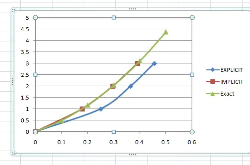
If we consider the above the graph it is evident that implicit method has given approx values compared to explicit.

In a more sophisticated convergence criteria may be necessary when solving
complex structures with many degrees of freedom. However, for this example problem minimization
of the norm of the residual is a sufficient criteria. It is important to note how
the initial increment due to the incremental load advances the solution forward. Then if an
implicit analysis is employed, Newton-Raphson iterations are used to make corrections to
the displacement in order to achieve equilibrium. Once satisfactory equilibrium is achieved,
a new load increment is applied to advance the solution and the process is repeated. Note
that an exact expression for force versus displacement is not always known.

Conclusion

A nonlinear analysis is illustrated using an incremental explicit and implicit procedure.
The results are plotted for comparison. It is evident from the results that the explicit analysis
drifts from the true solution. To overcome this problem an implicit analysis is used, which
includes Newton-Raphson iterations to enforce equilibrium between internal and external
forces. The techniques demonstrated are for a load control scheme. For other schemes such
as displacement control, arc length control and generalized displacement control the reader
is referred to the references given below. Many of the concepts and methods introduced are
similar to concepts and methods used in a nonlinear finite element analysis. Therefore, the
given example is a useful learning tool for students learning about methods of solution for
nonlinear problems.