Week 2 Air standard Cycle

Program:

import numpy as np

import matplotlib.pyplot as plt

# Constants

gamma = 1.4 # specific heat ratio for air

R = 0.287 # kJ/kg.K, specific gas constant for air

# Input parameters

compression_ratio = 8 # r = V1/V2

p1 = 100 # kPa

T1 = 300 # K

T3 = 2300 # K (peak temperature after combustion)

# State 1

v1 = 0.0005 # m^3 (initial volume)

v2 = v1 / compression_ratio

# Isentropic Compression (1 -> 2)

T2 = T1 * (compression_ratio)**(gamma - 1)

p2 = p1 * (compression_ratio)**gamma

# Constant Volume Heat Addition (2 -> 3)

v3 = v2

p3 = p2 * T3 / T2

T3 = T3

# Isentropic Expansion (3 -> 4)

v4 = v1

T4 = T3 * (1 / compression_ratio)**(gamma - 1)

p4 = p3 * (1 / compression_ratio)**gamma

# Constant Volume Heat Rejection (4 -> 1)

# returns to initial state

# Compute points for isentropic processes

def isentropic_process(p_start, v_start, v_end, gamma):

v = np.linspace(v_start, v_end, 100)

p = p_start * (v_start / v) ** gamma

return v, p

# Process 1-2 (Isentropic Compression)

v_12, p_12 = isentropic_process(p1, v1, v2, gamma)

# Process 2-3 (Constant Volume Heat Addition)

v_23 = [v2, v3]

p_23 = [p2, p3]

# Process 3-4 (Isentropic Expansion)

v_34, p_34 = isentropic_process(p3, v3, v4, gamma)

# Process 4-1 (Constant Volume Heat Rejection)

v_41 = [v4, v1]

p_41 = [p4, p1]

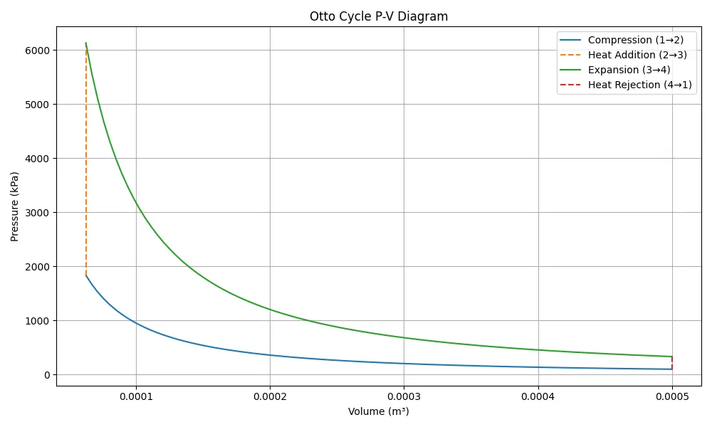
# Plotting the PV diagram

plt.figure(figsize=(10, 6))

plt.plot(v_12, p_12, label='Compression (1→2)')

plt.plot(v_23, p_23, label='Heat Addition (2→3)', linestyle='--')

plt.plot(v_34, p_34, label='Expansion (3→4)')

plt.plot(v_41, p_41, label='Heat Rejection (4→1)', linestyle='--')

plt.xlabel('Volume (m³)')

plt.ylabel('Pressure (kPa)')

plt.title('Otto Cycle P-V Diagram')

plt.grid(True)

plt.legend()

plt.tight_layout()

plt.show()

# Thermal Efficiency of Otto Cycle

efficiency = 1 - (1 / compression_ratio ** (gamma - 1))

print(f"Thermal Efficiency of Otto Cycle: {efficiency * 100:.2f}%")

Output: