Week 4.1 - Genetic Algorithm

function [f] = stalagmite(input_vector)
f1x = (sin(5.1*pi*input_vector(1)+0.5)).^6;
f1y = (sin(5.1*pi*input_vector(2)+0.5)).^6;
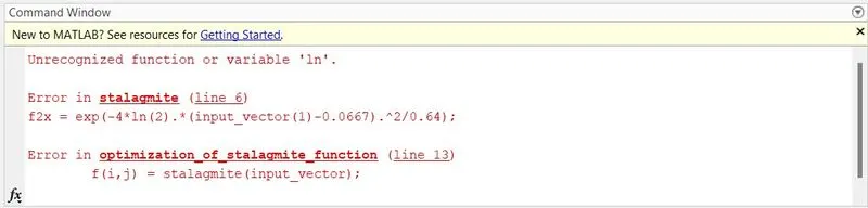
f2x = exp((-4*log(2)).*(input_vector(1)-0.0667)^2/(0.64));
f2y = exp((-4*log(2)).*(input_vector(2)-0.0667)^2/(0.64));
f = (f1x.*f1y.*f2x.*f2y);
end

clear all
close all
clc

% Inputs
x = linspace(0,0.6,150);
y = linspace(0,0.6,150);

% Here, Iteration are to be taken as 60.
iterations = 60;

% Creating a 2D Arrays
[xx,yy] = meshgrid(x,y);

% Assigning the values to the function variables
for i=1:length(xx)
    for j=1:length(yy)
        input_vector(1) = xx(i,j);
        input_vector(2) = yy(i,j);
        % Calling the Stalagmite function
        f(i,j) = stalagmite(input_vector);
    end
end

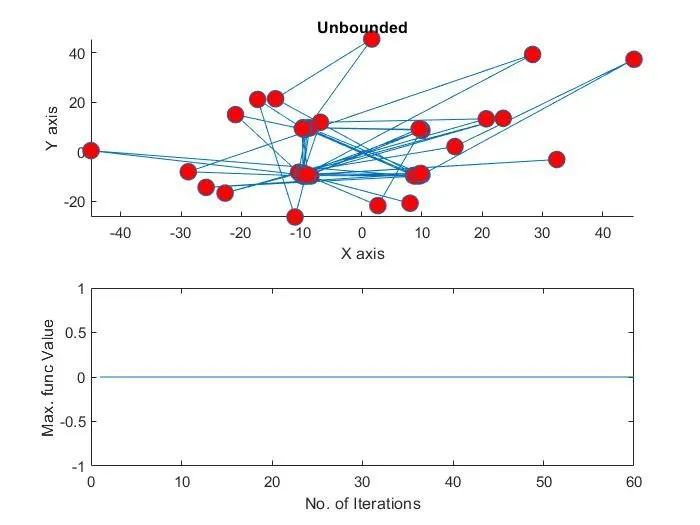
% Case-1 : Unbounded condition

% tic - toc is used to record the iteration period

tic

for i=1:iterations
    % [x, fval] = ga(func,nvars) - format
    [input,fval(i)] = ga(@stalagmite,2);    % ga is the one of the optimization process. 
    % Assigning the output variables
    xout(i) = input(1);
    yout(i) = input(2);
end

case_time_1=toc;

% Plots
figure(1);
subplot(2,1,1);
hold on;
surfc(xx,yy,f);
shading interp;
xlabel('X axis');
ylabel('Y axis');
plot3(xout,yout,fval,'marker','o','markersize',10,'markerfacecolor','r');
title('Unbounded','color','k');
subplot(2,1,2);
plot(fval);
xlabel('No. of Iterations');
ylabel('Max. func Value');

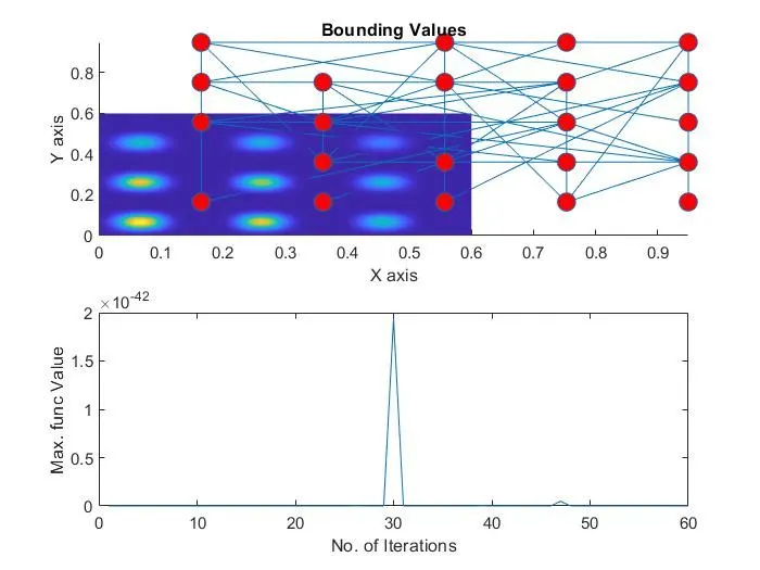
% Case-2 Bounding Values
tic

for i=1:iterations
    % [x,favl] = ga(func,nvars,A,b,Aeq,beq,lb,ub) - format
    % Here, set A=[],b=[],Aeq=[],beq=[] for no linear equalities
    [input,fval(i)] = ga(@stalagmite,2,[],[],[],[],[0;0],[1;1]);
    xout(i) = input(1);
    yout(i) = input(2);
end

case_time_2=toc;

% plots
figure(2);
subplot(2,1,1);
hold on;
surfc(xx,yy,f);
shading interp;
xlabel('X axis');
ylabel('Y axis');
plot3(xout,yout,fval,'marker','o','markersize',10,'markerfacecolor','r');
title('Bounding Values','color','k');
subplot(2,1,2);
plot(fval);
xlabel('No. of Iterations');
ylabel('Max. func Value');

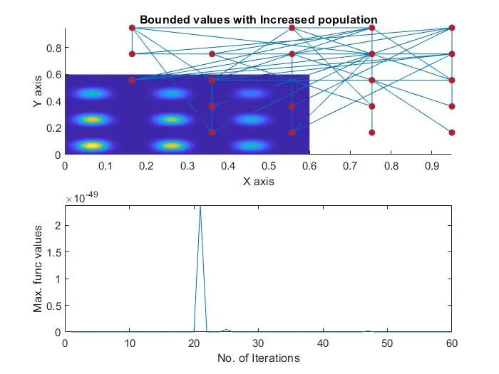
% Case-3 Bounding values and increasing the population

% For initialize the population, use 'optimoptions' command
options = optimoptions('ga');
options = optimoptions(options,'populationsize',300);

tic

for i = 1:iterations
    % [x,fval] = ga(func,nvars,A,b,Aeq,beq,lb,ub,nonlcon,options) - format
    % Here, set A=[],b=[],Aeq=[],beq=[] for no linear equalities
    [input,fval(i)] = ga(@stalagmite,2,[],[],[],[],[0;0],[1;1],[],[],options);
    xout(i)=input(1);
    yout(i)=input(2);
end

case_time_3 = toc;

% Plots
figure(3);
subplot(2,1,1);
hold on;
surfc(xx,yy,f);
shading interp;
xlabel('X axis');
ylabel('Y axis');
plot3(xout,yout,fval,'marker','o','markersize',5,'markerfacecolor','r');
title('Bounded values with Increased population');
subplot(2,1,2);
plot(fval);
xlabel('No. of Iterations');
ylabel('Max. func values');

https://drive.google.com/file/d/1u1bpkkVXTcv1aSzwERvbrXREzM4r6xkQ/view?usp=drivesdk

https://drive.google.com/file/d/1tyialBaH3QBXgBNxfVXeW3gSMh2OWsAD/view?usp=drivesdk