Week 2 Air standard Cycle
AIM:- Based on the concepts you have learnt during the forward kinematics routine, go ahead and write code that can solve an otto cycle and make plots for it.
Here are the requirements
1. Your code should create a PV diagram
2. You should output the thermal efficiency of the engine.
Once you have done this, create a project in projects.skill-lync.com.
Use the "INSERT CODE SAMPLE" option to paste your code and attach screenshots of the output.
The Otto cycle is a thermodynamic process that explains the transformation of gasoline's chemical energy into thermal energy within spark ignition internal combustion engines. It involves a series of pressure, temperature, volume, and heat exchange changes, ultimately converting fuel into motion. This cycle is utilized in both 2-stroke and 4-stroke engine configurations.
Nikolaus August Otto, a German Engineer, involved himself in the study of heat engines and built his first working four-stroke engine in 1876. Coal gas and air mixture were used as working fluid. Wilhelm Maybach joined Otto to revamp the model based on Otto’s theory and made an engine called Otto Engine.
A revision of this engine was made that changed the way the whole world was functioning
It helps us study the changes in pressure, temperature, and rate of heat flow of the fluid in the system. The Otto cycle has several processes which are studied using the P-v and T-s diagrams in the later sections.
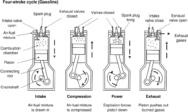
P-v Diagram for Otto Cycle
The pressure-volume diagram is given below which we will use to understand the processes involved in the cycle.
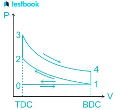
Fig 1: Otto Cycle Pv Diagram
To study the processes referring to the P-v diagram above, let us assume that we are speaking about IC engines.
(1) Process 0 - 1: Air at constant pressure is drawn into the piston-cylinder arrangement.
(2) Process 1 - 2: The piston moves from the bottom dead centre (BDC) to the top dead centre (TDC) compressing the fuel and air (charge) in an adiabatic compression.
(3) Process 2 - 3: The heat is transferred from an external source at a constant volume to the charge while the piston is still at the TDC. The mixture rapidly burns in this process
(4) Process 3 - 4: When the mixture burns, it expands adiabatically or isentropically. This is called the power stroke.
(5) Process 4 - 1: The heat is rejected from the air at constant volume at the end of the cycle. The piston will be at the BDC in this process.
(6) Process 1 - 0: This is the exhaust stroke where the mixture is released into the atmosphere.
FORMULA
The formula to find volume is given below.
The formula to find thermal efficiency is given below
Here the term k is denoted as gamma in the program
r is denoted as cr in the program
PROCEDURE
- Since the otto cycle is an air standard cycle we will take the gamma value as 1.4.
- At the initial condition, we will consider the T1 and P1 values as 500K and 101.325KPa respectively.
- The geometrical parameters are stoke, diameter, connecting rod length, crank start and end angle are defined to the function in the program.
- From the above parameters, the v_c and v_s are calculated accordingly.
- The other states are calculated using adiabatic and ideal gas equations.
- Similarly, the thermal efficiency is calculated using the above formulas.
- For plotting p-v diagram plt.plot command is used from matplotlib.pyplot module.
- For the compression stage, the starting and ending crank angles are 180 and 0.
- For the expansion stage, the starting and ending crank angles are 0 and 180.
- Let us consider the value to be iterated is 50 accordingly v null set is created to store the value using append command.
Programme:-
import math
import matplotlib.pyplot as plt
def Engine_kinematics(bore, stroke, con_rod, CR, start_crank, end_crank):

    #engine parameters
	a = stroke/2
	R = con_rod/a

	v_s = (math.pi/4) * pow(bore,2) * stroke
	v_c = v_s/(CR -1)

	sc = math.radians(start_crank)
	ec = math.radians(end_crank)

	num_values = 50

	dtheta = (ec-sc)/(num_values - 1)

	V = []

	for i in range (0,num_values):
		theta = sc + i * dtheta
		term1 = 0.5*(CR-1)
		term2 = R + 1-math.cos(theta)
		term3 = pow(R,2) - pow(math.sin(theta),2)
		term3 = pow(term3,0.5)
		V.append((1+term1*(term2-term3))*v_c)

	return V

# Inputs
p1 = 101325
t1 = 500
gamma = 1.4
t3 = 2300

#Geomentric parameter
bore = 0.1
stroke = 0.1
con_rod = 0.15
CR = 12

#volume computation
V_s = (math.pi/4) * pow(bore,2)*stroke
V_c = V_s/(CR-1)
v1 = V_s + V_c

#state point 2
v2 = V_c

# p2v2^gamma = p1v1^gamma
p2 = p1*pow(v1,gamma)/pow(v2,gamma)

#p2v2/t2 = p1v1/t1 | rhs = p1v1/t1 | p2v2/t2 = rhs | t2 = p2v2/rhs
rhs = p1*v1/t1
t2 = p2*v2/rhs

V_compression  = Engine_kinematics(bore, stroke, con_rod, CR, 180, 0)
constant = p1*pow(v1,gamma)
P_compression = []
for V in V_compression:
	P_compression.append(constant/pow(V,gamma))

# state point 3
v3 = v2

# p3v3/t3 = p2v2/t2 | rhs = p2v2/t2 | p3 = rhs*t3/v3
rhs = p2*v2/t2
p3 = rhs*t3/v3
V_expansion  = Engine_kinematics(bore, stroke, con_rod, CR, 0, 180)
constant = p3*pow(v3,gamma)
P_expansion = []
for V in V_expansion:
	P_expansion.append(constant/pow(V,gamma))

# State point 4
v4 = v1

#p4v4^gamma = p3v3^gamma
p4 = p3*pow(v3, gamma)/pow(v4, gamma)

#p4v4/t4 = rhs
t4 = p4*v4/rhs

plt.plot([v2,v3],[p2,p3])
plt.plot(V_compression,P_compression)
plt.plot(V_expansion,P_expansion)
plt.plot([v4,v1],[p4,p1])
plt.xlabel('volume')
plt.ylabel('pressure')
plt.title('pressure vs volume')

#thermal efficiency
thermal_efficiency = 1-(1/(pow(CR,(gamma-1))))
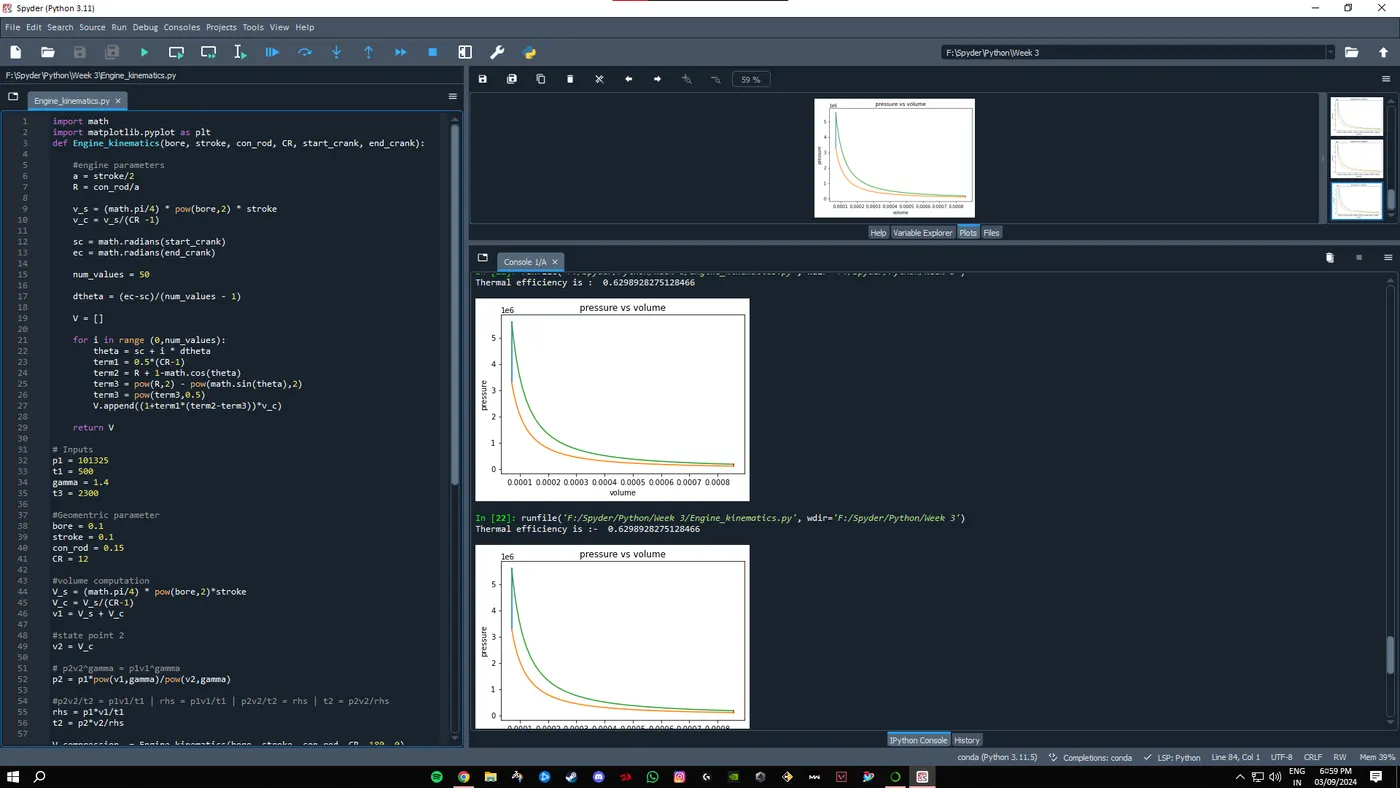
print ('Thermal efficiency is :- ',thermal_efficiency)
import math
import matplotlib.pyplot as plt
def Engine_kinematics(bore, stroke, con_rod, CR, start_crank, end_crank):
#engine parameters
a = stroke/2
R = con_rod/a
v_s = (math.pi/4) * pow(bore,2) * stroke
v_c = v_s/(CR -1)
sc = math.radians(start_crank)
ec = math.radians(end_crank)
num_values = 50
dtheta = (ec-sc)/(num_values - 1)
V = []
for i in range (0,num_values):
theta = sc + i * dtheta
term1 = 0.5*(CR-1)
term2 = R + 1-math.cos(theta)
term3 = pow(R,2) - pow(math.sin(theta),2)
term3 = pow(term3,0.5)
V.append((1+term1*(term2-term3))*v_c)
return V
# Inputs
p1 = 101325
t1 = 500
gamma = 1.4
t3 = 2300
#Geomentric parameter
bore = 0.1
stroke = 0.1
con_rod = 0.15
CR = 12
#volume computation
V_s = (math.pi/4) * pow(bore,2)*stroke
V_c = V_s/(CR-1)
v1 = V_s + V_c
#state point 2
v2 = V_c
# p2v2^gamma = p1v1^gamma
p2 = p1*pow(v1,gamma)/pow(v2,gamma)
#p2v2/t2 = p1v1/t1 | rhs = p1v1/t1 | p2v2/t2 = rhs | t2 = p2v2/rhs
rhs = p1*v1/t1
t2 = p2*v2/rhs
V_compression = Engine_kinematics(bore, stroke, con_rod, CR, 180, 0)
constant = p1*pow(v1,gamma)
P_compression = []
for V in V_compression:
P_compression.append(constant/pow(V,gamma))
# state point 3
v3 = v2
# p3v3/t3 = p2v2/t2 | rhs = p2v2/t2 | p3 = rhs*t3/v3
rhs = p2*v2/t2
p3 = rhs*t3/v3
V_expansion = Engine_kinematics(bore, stroke, con_rod, CR, 0, 180)
constant = p3*pow(v3,gamma)
P_expansion = []
for V in V_expansion:
P_expansion.append(constant/pow(V,gamma))
# State point 4
v4 = v1
#p4v4^gamma = p3v3^gamma
p4 = p3*pow(v3, gamma)/pow(v4, gamma)
#p4v4/t4 = rhs
t4 = p4*v4/rhs
plt.plot([v2,v3],[p2,p3])
plt.plot(V_compression,P_compression)
plt.plot(V_expansion,P_expansion)
plt.plot([v4,v1],[p4,p1])
plt.xlabel('volume')
plt.ylabel('pressure')
plt.title('pressure vs volume')
#thermal efficiency
thermal_efficiency = 1-(1/(pow(CR,(gamma-1))))
print ('Thermal efficiency is :- ',thermal_efficiency)