Week 2 Air standard Cycle

AIR STANDARD CYCLE USING PYTHON

AIM

            To write a program in python to solve the otto cycle and plot the graph.

OBJECTIVE

1. To solve different state variables in the otto cycle and plot p-v diagram.
2. To calculate thermal efficiency for the given parameters in the otto cycle.

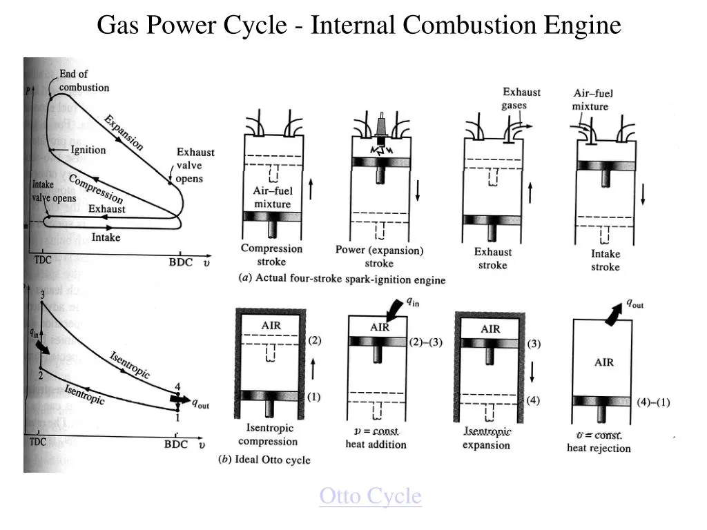
PROCESS IN OTTO CYCLE

• Process 0–1 a mass of air is drawn into piston/cylinder arrangement at constant pressure.
• Process 1–2 is an adiabatic (isentropic) compression of the charge as the piston moves from the bottom dead center(BDC) to the top dead center (TDC).
• Process 2–3 is a constant-volume heat transfer to the working gas from an external source while the piston is at the top dead center. This process is intended to represent the ignition of the fuel-air mixture and the subsequent rapid burning.
• Process 3–4 is an adiabatic (isentropic) expansion (power stroke).
• Process 4–1 completes the cycle by a constant-volume process in which heat is rejected from the air while the piston is at the bottom dead center.
• Process 1–0 the mass of air is released to the atmosphere in a constant pressure process.

The Otto cycle consists of isentropic compression, heat addition at constant volume, isentropic expansion, and rejection of heat at constant volume. In the case of a four-stroke Otto cycle, technically there are two additional processes: one for the exhaust of waste heat and combustion products at constant pressure (isobaric), and one for the intake of cool oxygen-rich air also at constant pressure; however, these are often omitted in a simplified analysis. Even though those two processes are critical to the functioning of a real engine, wherein the details of heat transfer and combustion chemistry are relevant, for the simplified analysis of the thermodynamic cycle, it is more convenient to assume that all of the waste heat is removed during a single volume change.

FORMULA

The formula to find volume is given below.

The formula to find thermal efficiency is given below

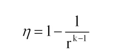
Here the term k is denoted as gamma in the program

r is denoted as cr in the program

PROCEDURE

• Since the otto cycle is an air standard cycle we will take the gamma value as 1.4.
• At the initial condition, we will consider the T1 and P1 values as 500K and 101.325KPa respectively.
• The geometrical parameters are stoke, diameter, connecting rod length, crank start and end angle are defined to the function in the program.
• From the above parameters, the v_c and v_s are calculated accordingly.
• The other states are calculated using adiabatic and ideal gas equations.
• Similarly, the thermal efficiency is calculated using the above formulas.
• For plotting p-v diagram plt.plot command is used from matplotlib.pyplot module.
• For the compression stage, the starting and ending crank angles are 180 and 0.
• For the expansion stage, the starting and ending crank angles are 0 and 180.
• Let us consider the value to be iterated is 50 accordingly v null set is created to store the value using append command.

PROGRAM

# otto cycle simulator


import math
import matplotlib.pyplot as plt

def engine_kinematics(bore, stroke, con_rod, cr, start_crank, end_crank):


	# Geometic parametrs
	a = stroke/2
	R = con_rod/a

	# volume computation
	v_s = (math.pi/4)*pow(bore,2)*stroke
	v_c = v_s/(cr-1)

	sc = math.radians(start_crank)
	ec = math.radians(end_crank)

	num_values = 50 

	dtheta = (ec-sc)/(num_values-1)

	v = []

	for i in range(0,num_values):
		theta = sc + i*dtheta
		term1 = 0.5*(cr-1)
		term2 = R + 1 - math.cos(theta)
		term3 = pow(R,2) - pow(math.sin(theta),2)
		term3 = pow(term3,0.5)

		v.append((1 + term1*(term2 - term3))*v_c)

	return v
	

# inputs 
p1 = 101325
t1 = 500
gamma = 1.4
t3 = 2300

# geometric parameters
bore = 0.1
stroke = 0.1
con_rod = 0.15
cr = 12

# volume computation

v_s = (math.pi/4)*pow(bore,2)*stroke
v_c = v_s/(cr-1)
v1 = v_c + v_s

# state point 2
v2 = v_c

# p2v2^gamma = p1v1^gamma
p2 = p1*pow(v1,gamma)/pow(v2,gamma)

#p2v2/t2 = p1v1/t1 | rhs = p1v1/t1 | p2v2/t2 = rhs | t2 = p2v2/rhs
rhs = p1*v1/t1
t2 = p2*v2/rhs

v_compression = engine_kinematics(bore, stroke, con_rod, cr, 180,0)

constant = p1*pow(v1,gamma)

p_compression = []

for v in v_compression:
	p_compression.append(constant/pow(v,gamma))
	

# state poinnt 3
v3 = v2

#p3v3 =p2v2/t2 | rhs = p2v2/t2 | p3 = rhs*t3/v3

rhs = p2*v2/t2
p3 = rhs*t3/v3

v_expansion = engine_kinematics(bore, stroke, con_rod, cr, 0,180)

constant = p3*pow(v3,gamma)

p_expansion = []

for v in v_expansion:
	p_expansion.append(constant/pow(v,gamma))

#state point 4
v4 = v1

# p4v4^gamma = p3v3^gamma
p4 = p3*pow(v3,gamma)/pow(v4,gamma)

# p4v4/t4 = rhs

t4 = p4*v4/rhs 

plt.plot([v2,v3],[p2,p3])
plt.plot(v_compression, p_compression)
plt.plot(v_expansion, p_expansion)
plt.plot([v4,v1],[p4,p1])
plt.xlabel('Volume(m^3)')
plt.ylabel('Pressure(pa)')
plt.title('P-V diagram of an otto cycle')
plt.show()

# Thermal effiency
n = 1 - (pow(cr,(1-gamma)))
print(n)

OUTPUT

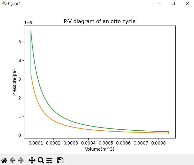
The p-v diagram for the otto cycle

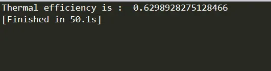
The thermal efficiency is 62.9%

CONCLUSION

            The desired p-v diagram of the otto cycle is plotted using python programming language by using an array of volume and different crank angles.