Week 4.1 - Genetic Algorithm

Aim : To optimise the stalagmite function and to find the global maxima of the function.

Introduction :

The genetic algorithem is a method for solving both constrained and unconstrained optimization problems that is based on nature selection. The genetic algorithm repeatdly modifies a population of individual solutions. A genetic algorithm is a search heuristic that is inspired by Charless Darwins's theory of natural evaluation.

Code to stalagmite function and to find global maximum of the function :

code 1:

% creating the genetic alogorithm code

clear all
close all
clc

% Defining our search space
x = linspace(0,0.6,150);
y = linspace(0,0.6,150);

% Creating a 2Dimensional mesh
[xx yy] = meshgrid(x,y);

% Evaluating the stalagmite function
for i = 1:length(xx)
    for j = 1:length(yy)
        input_vector(1)=xx(i,j);
        input_vector(2)=yy(i,j);
        f(i,j) = stalagmite(input_vector);
    end
end


surfc(xx,yy,f)
xlabel('x value')
ylabel('y value')

shading interp

[inputs,fval] = ga(@stalagmite,2)

Tthe above program is used to craete a stalagmite function by passing the input arrays as the argument for the variables x and y. The output is obtained by using the function.

• we start with the clear all , close all, clc command.
• 2 dimensional mesh is created by using meshgrid.
• first loop is for the xx variables = i = l:length(xx).
• second loop is for the yy variables = j =l:length(yy).
• 'surf' command is used for getting the smooth plot.
• 'shading interp' is used for the plot to clear plot.

Function code :

% stalagmite function code

function [f] = stalagmite(input_vector)

f1 = (sin(5.1*pi * input_vector(1) + 0.5))^6;
f2 = (sin(5.1*pi * input_vector(2) + 0.5))^6;
f3 = exp(-4*log(2)*(input_vector(1)-0.0667)^2/0.64);
f4 = exp(-4*log(2)*(input_vector(2)-0.0667)^2/0.64);
f = -(f1*f2*f3*f4);
end

we give the formula for the inputs as f1,f2,f3,f4

Main code :

% main code

clear all
close all
clc

% Defining our search space
x = linspace(0,0.6,150);
y = linspace(0,0.6,150);
num_case = 50;

% Creating a 2Dimensional mesh
[xx yy] = meshgrid(x,y);

% Evaluating the stalagmite function
for i = 1:length(xx)
    for j = 1:length(yy)
        input_vector(1)=xx(i,j);
        input_vector(2)=yy(i,j);
        f(i,j) = stalagmite(input_vector);
    end
end

% study 1 - statistical behaviour

tic 
for i = 1:num_case
    [inputs,fopt(i)] = ga(@stalagmite,2);
    xopt(i) = inputs(1);
    yopt(i) = inputs(2);
end
fopt = -fopt;
study_time = toc

figure(1)
subplot(2,1,1)
hold on
surfc(x,y,-f)
shading interp
plot3(xopt,yopt,fopt,'marker','o','MarkerSize',5,'MarkerFaceColor','r')
title('unbounded inputs')
subplot(2,1,2)
plot(fopt)
xlabel('interations')
ylabel('function minimum')

tic
%stdy 2 - statistical behaviour  with upper and lower bound

for i = 1:num_case
    [inputs,fopt2(i)] = ga(@stalagmite,2,[],[],[],[],[0;0],[1;1]);
    xopt2(i) = inputs(1);
    yopt2(i) = inputs(2);
end
fopt2 = -fopt2
study2_time = toc

figure(2)
subplot(2,1,1)
hold on
surfc(x,y,-f)
shading interp
plot3(xopt2,yopt2,fopt2,'marker','o','MarkerSize',5,'MarkerFaceColor','r')
title('bounded inputs')
subplot(2,1,2)
plot(fopt2)
xlabel('interations')
ylabel('function minimum')

%study 3 increasing ga interations
options = optimoptions('ga');
options = optimoptions(options,'populationsize',300);

tic
for i = 1:num_case
    [inputs3,fopt3(i)] = ga(@stalagmite,2,[],[],[],[],[0,0],[1,1],[],[],options);
    xopt3(i) = inputs3(1);
    yopt3(i) = inputs3(2);
end

study3_time = toc

figure(3)
subplot(2,1,1)
hold on
surfc(x,y,-f)
shading interp
plot3(xopt3,yopt3,fopt3,'marker','o','MarkerSize',5,'MarkerFaceColor','r')
title('bounded inputs')
subplot(2,1,2)
plot(-fopt3)
xlabel('interations')
ylabel('function minimum')

Here we use the 3 study cases :

• Study 1 as a statistical behaviour.
• Study 2 as a statistical behaviour with upper and lower boundaries.
• Study 3 as increasing ga interactions.

Study 1:

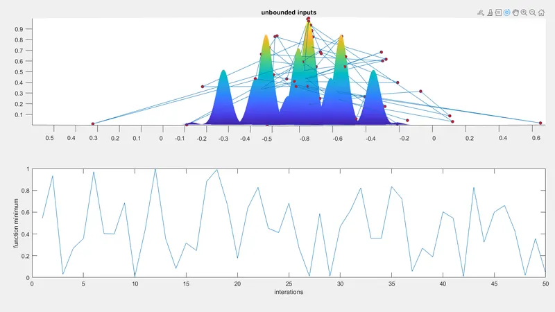
The program in study 1 is for statistical behaviour of the unbounded inputs.

xopt is the input(1)

yopt is the input(2)

syntax of GA = ga(@stalagmite,2)

tic and tac is used for creating the study time.

Study 2:

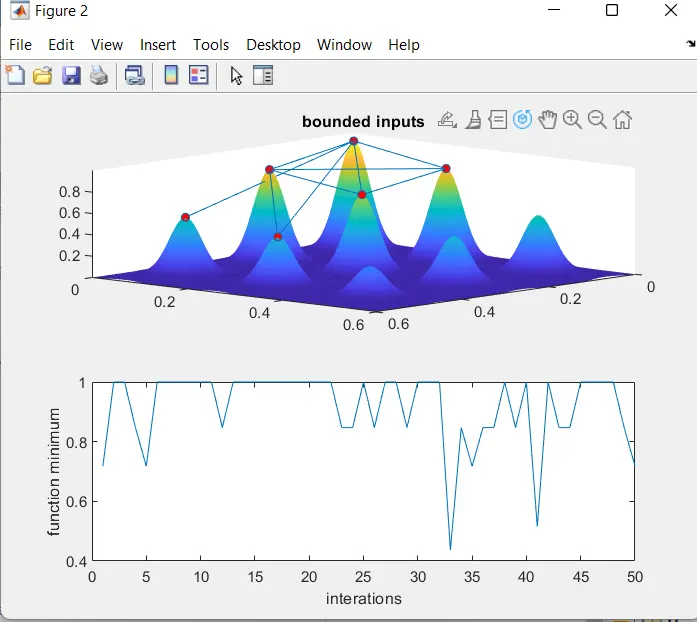
The study 2 deals with statistical behaviour of the bounded inputs.

syntax of GA = ga(@stalagmite,2,[],[],[],[],[])

Tic and is used for creating the study time.

Study 3:

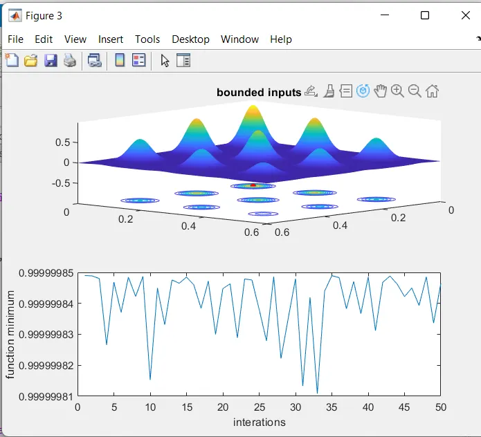
The global maxima is obtained by increasing the population size.

syntax of GA = ga(@stalagmite,2,[],[],[],[],[],options)

Tic and is used for creating the study time.

plot1 (or) figure1:

plot2 (or) figure2 :

plot3 (or) figure3:

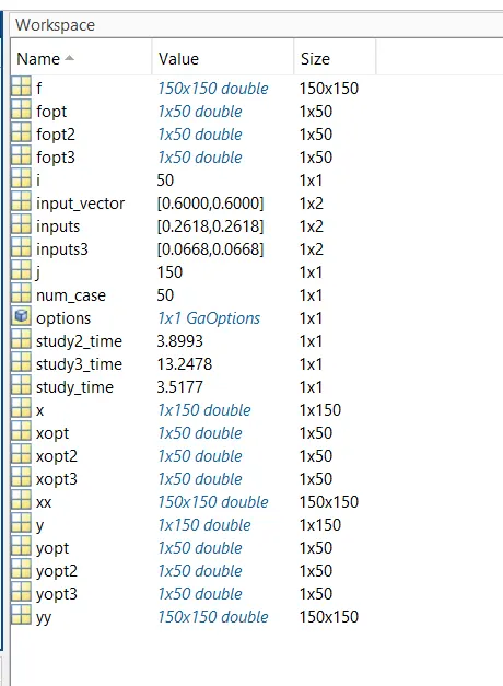
Work space :

Conclusion :

The global maxima is calculated by population sizing and the plots provided a visual context of the solution and verifies the authentical of the obtained values.