Week 3 - Solving second order ODEs

Aim: To create the animation of simple pendulum by using second order differential equation and also to plot graph between angular velocity and displacement.

Theory: A simple pendulum is a weight suspended from a pivot, so that it can swing freely. It consists of a mass rod, frictionless pivot or point of suspension, angular displacement, bob.

Equation:

d^2(theta)/dt^2+b/m*d(theta)/dt+g/l*sin(theta)

here,

• l = lenth = 1 meter
• b = damping = 0.05
• m = mass = 1kg
• g = gravity = 9.81 m/s^2

Code expanation :

• we start the code with clear all, close all, clc.
• We give the intial conditions.
• next we give the intial points
• we slove the ode's.
• we plot the results and we give the xlabels and ylabels.
• Then we Animate the transit mtion of the simple pendulum motion.
• Finally,we start making video of simple pendulum.

Code :

% Animation of the transit motion of the simple pendulum.

clear all
close all
clc

b=0.02;
g=9.81;
l=1;
m=0.1;

%initial condition
theta_0 = [0;5];

%time points
t_span = linspace(0,20,500);

%solve ode
[t , results] = ode45(@(t,theta) ode_func(t,theta,b,g,l,m),t_span,theta_0);

figure (1)

plot(t,results(:,1))
hold on
plot(t,results(:,2))
ylabel('plot')
xlabel('time')


ct=1;
figure(2)
for i = 1:length(results(:,1));
    x0 = 0;
    y0 = 0;
    x1 = l*sin(results(i,1));
    y1 = -1*cos(results(i,1));

    plot([-1.5 1.5],[0 0])
    hold on

    plot([x0 x1],[y0 y1],'LineWidth',3,'Color','b')
    axis([-2 2 -2 2])

    plot(x1,y1,'o','markersize',20,'Color','r')
    pause(0.001)
    grid on
    M(ct) = getframe(gcf)
    hold off

    ct = ct+1
end

% making the file video

movie(M)
videofile = VideoWriter('simple pendulum.avi')
open(videofile)
writeVideo(videofile,M)
close(videofile)

Function code:

function [dtheta_dt] = ode_func(t,theta,b,g,l,m)

       theta1 = theta(1)
       theta2 = theta(2)
       dtheta1_dt = theta2;
       dtheta2_dt = -(b/m)*theta2 - (g/l)*sin(theta1);
       dtheta_dt = [dtheta1_dt ; dtheta2_dt];

end       

Plot :

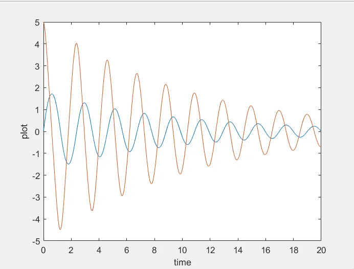
Animation video:

https://youtu.be/UEv5AFnwuz8

Errors occured :

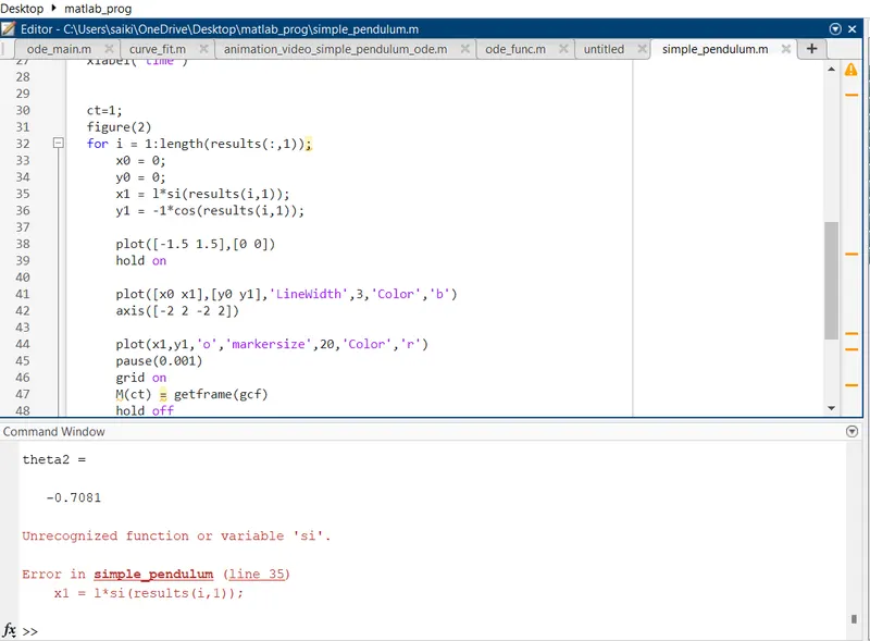
Solution : The error can be solved by giving the value 'sin' in the line35.