Week 2 Air standard Cycle

import math #The math module is used to use mathematical functions
import matplotlib.pyplot as plt #module used to plot graphs

#defining the function 
def enginekinematics (bore , stroke , conn_rod, cr, crank_start , crank_end): #crank_start and crank_end are the starting and the ending crank angles of the crank shaft during cumbustion process 
	
	cpr = stroke/2 #crank pin radius
	R = conn_rod/cpr 

	#volume parameters 
	V_stroke = math.pi*(1/4)*pow(bore,2)*stroke #Swept volume
	V_clearence = V_stroke/(cr-1) #Clearance volume


	sc= math.radians(crank_start) #defines the angle of the starting crank depending upon the input value givin while calling the functiom
	ec= math.radians(crank_end) #defines the angle of the ending crank depending upon the input value givin while calling the functiom
	
	num_val = 50

	bw_angle = (ec-sc)/(num_val-1) #crank angle spacing 

	V=[]

	for i in range (0,num_val):
		theta = sc + i*bw_angle
		term1 = 0.5*(cr - 1)
		term2= R + 1 - math.cos(theta)
		term3= pow(R,2) - pow (math.sin(theta),2)
		term3 = pow(term3, 0.5 )

		V.append((1 + term1*(term2 - term3))*V_clearence)
		
	return V

#initial conditions 
p1 = 101325
t1 = 500
gamma = 1.4
t3 = 2300

#geo para
bore = 0.10 
stroke = 0.1
conn_rod = 0.15 #connecting rod length in meters
cr= 8 #compression ratio
cpr = stroke/2 #crank pin radius
R = conn_rod/2

#vol computation 
v_swept = (math.pi/4)*pow(bore,2)*stroke #Swept volume
v_clearance = v_swept/(cr-1) #Clearance volume	
v1 = v_clearance + v_swept #total volume

#stage 2 
v2 = v_clearance #at stage two volume in the combustion chamber is equal to clearance volume

#to compute pressure p2*v2^gamma =p1v1^gamma 
p2 = p1*pow(v1,gamma)/pow(v2,gamma)

#to compute temperature at stage 2 p2v2/t2 = p1v1/t1
rhs = p1*v1/t1
t2 = p2*v2/rhs #since rhs = p1*v1/t1
V_compression = enginekinematics (bore , stroke , conn_rod,cr , 180,0) #compression process takes place since theta is going from 180-0

constant = p1*pow(v1,gamma)

P_compression = []

for v in V_compression:
	P_compression.append(constant/pow(v,gamma)) 


#stage 3
v3 = v2 #contant heat addition 

#to compute pressure at state 3. p2v2/t2 = p3v3/t3  
rhs = p2*v2/t2
p3 = rhs*t3/v3

V_expansion = enginekinematics (bore , stroke , conn_rod,cr , 0,180) #expansion process takes place since theta is going from 0-180

constant = p3*pow(v3,gamma)

P_expansion = []

for v in V_expansion:
	P_expansion.append(constant/pow(v,gamma)) 

#stage 4
v4=v1

#p4v4^gamma = p3v3^gamma
p4 = p3*pow(v3,gamma)/pow(v4,gamma)

#p4v4/t4 = p3v3/t3 #rhs = p4*v4/t4

t4 = p4*v4/rhs

#calculating the thermal efficiency 
thermal_efficiency = (1-(1/pow(cr,gamma - 1)))*100
print('thermal efficiency =', thermal_efficiency)


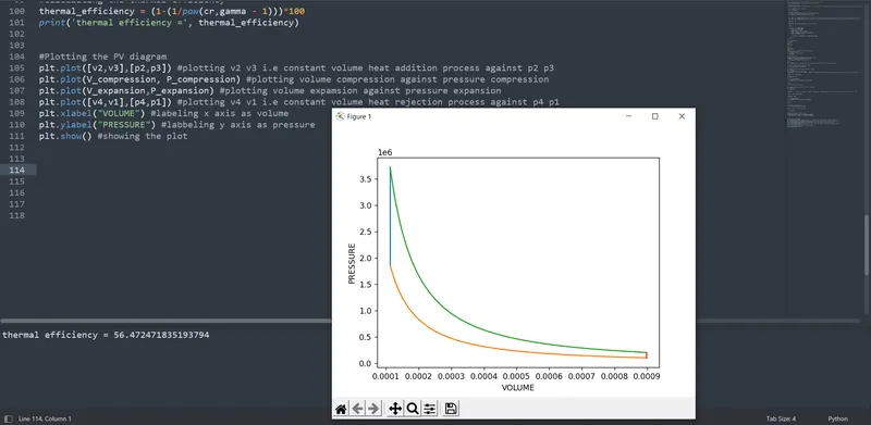
#Plotting the PV diagram 
plt.plot([v2,v3],[p2,p3]) #plotting v2 v3 i.e constant volume heat addition process against p2 p3
plt.plot(V_compression, P_compression) #plotting volume compression against pressure compression
plt.plot(V_expansion,P_expansion) #plotting volume expamsion against pressure expansion
plt.plot([v4,v1],[p4,p1]) #plotting v4 v1 i.e constant volume heat rejection process against p4 p1
plt.xlabel("VOLUME") #labeling x axis as volume	
plt.ylabel("PRESSURE") #labbeling y axis as pressure 
plt.show() #showing the plot

Program output