Week 6 - Data analysis

import matplotlib.pyplot as plt #module used to plot graphs
import math #The math module is used to use mathematical functions
import numpy as np #used for scientific computing
from scipy.integrate import simps #scipy module provides more utility functions for optimization 

#Compatibility check
file_name = input("Enter the filename: ")

if file_name == 'engine_data.out': #checking if the file name exists with if loop
	print("File is recognized. Please proceed furter.")
else:
	print("File not recognized. Please provide a valid CONVERGE output file")

	exit()

line_count = 1 #Keeping a track of lines by taking one line at a time

print('Press the respective number for respective parameter output') #The 16 parameters have 16 respective codes, select the codes from the following
parameter_num = ['crank_angle=0','pressure=1','max_pres=2','min_pres=3','mean_temp=4','max_temp=5','min_temp=6','volume=7','mass=8','density=9','Heat Rejection=10','Heat Rejection=11','C_p=12','C_v=13','gamma=14','Kinematic Viscosity=15','Dynamic Viscosity=16']
print(parameter_num)

first_column=int(input('Enter the first column:')) #entering the first column number	
second_column=int(input('Enter the second column:')) #entering the second column number
print('\n') #leaving a line 


column_1=[] #creating an empty array for colomn 1 values
column_2=[] #creating an empty array for colomn 1 values

for line in open('engine_data.out'): #opening the file that contains a particular data and reading each and every line of that file
	if'#' not in line: 
		column_1.append(float(line.split()[first_column-1])) #adding value to the column_1 array
		column_2.append(float(line.split()[second_column-1])) ##adding value to the column_2 array

		line_count+=1

area=float(simps(column_1, column_2)) #Simpson method is used to calculate the area under the PV diagram by using the algorith of scipy.integrate import simps
print('area:{}\n' .format(area))


rpm=1500 #rpm value
speed=rpm/60 #speed value
power=area*speed #formula for calculating power
print('power:{} \n' .format(power))

mass_of_fuel = 20*pow(10,-6) #formula for calculating the mass of the fuel
sfc =mass_of_fuel/power #formula for calculating specific fuel consumption 
print('specific fuel consumption: {}\n'.format(sfc)) 

parameters = ['Crank Angle=0','Pressure','Max pressure','Min presssure ','Mean temperature ','Max Temperature','Min temperature ','Volume','Mass ','Density ','Heat Rejection ','Heat Rejection ','Cp=12','Cv=13','Gamma','Kinematic Viscosity','Dynamic Viscosity']
units = ['(DEG)','(Mpa)','(Mpa)','(Mpa)','(K)','(K)','(K)','pow(m,3)','(kg)','(kg/(pow(m,3))','(J)','(J)','(J/time)','(J/kgK)','(J/kgK)','','pow(m,2)/s','(Ns/pow(m,2)']

#plotting the graph 
plt.plot(column_2,column_1 ,linewidth=3,color='blue') #plotting the graph between column 1 and column 2
plt.xlabel(parameters[first_column] + ' ' + units[first_column] ,color='green',fontsize=12) #labeling the x axis of the graph
plt.ylabel(parameters[second_column] + ' ' + units[second_column] ,color='green',fontsize=12) #labeling the y axis of the graph
plt.title(parameters[first_column] + '  VS  ' + parameters[second_column],color='orange',fontsize=15) #giving the title of to the graph
plt.savefig(parameters[first_column] + 'VS' + parameters[second_column] + '.png') #saving the graph as a figure  
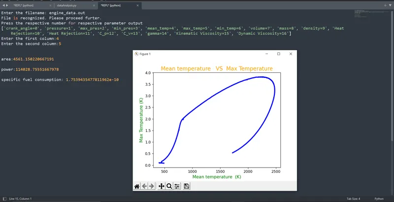
plt.show() #showcasing the file

OUTPUT: