Week 3 - Solving second order ODEs

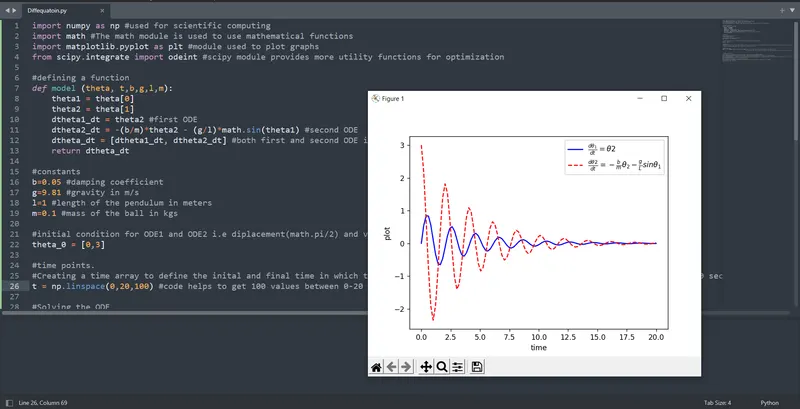
import numpy as np #used for scientific computing
import math #The math module is used to use mathematical functions 
import matplotlib.pyplot as plt #module used to plot graphs 
from scipy.integrate import odeint #scipy module provides more utility functions for optimization 

#defining a function
def model (theta, t,b,g,l,m):
	theta1 = theta[0]
	theta2 = theta[1]
	dtheta1_dt = theta2 #first ODE
	dtheta2_dt = -(b/m)*theta2 - (g/l)*math.sin(theta1) #second ODE
	dtheta_dt = [dtheta1_dt, dtheta2_dt] #both first and second ODE in one ODE 
	return dtheta_dt

#constants
b=0.05 #damping coefficient 
g=9.81 #gravity	in m/s
l=1 #length of the pendulum in meters
m=0.1 #mass of the ball in kgs

#initial condition for ODE1 and ODE2 i.e diplacement(math.pi/2) and velocity(0)
theta_0 = [0,3]

#time points.
#Creating a time array to define the inital and final time in which the the pendulum simulates. Here inital time is 0 and final time is 20 seconds
t = np.linspace(0,20,100) #code helps to get 100 values between 

#Solving the ODE
theta = odeint(model, theta_0,t,args =(b,g,l,m)) #odeint is a function thats gonna intigrate the system of ODE.
                                                 #to intigrate the ODE, we need to define the initial conditions like model, thera_0,time,arguments i.e b,g,l,m


#plotting the results
#since theta is the solution vector it contains 2 rows i.e 0,1 and multiple columns. 
plt.plot(t,theta[:,0],'b-',label=r'$\frac{d\theta_1}{dt}=\theta2$') #solution for first ODE i.e displacement 
plt.plot(t,theta[:,1],'r--',label=r'$\frac{d\theta2}{dt}=-\frac{b}{m}\theta_2-\frac{g}{L}sin\theta_1$') #solution for seconf ODE i.e vellocity
plt.ylabel('plot') #labeling the y axis of the graph
plt.xlabel("time") #labeling the x axis of the graph
plt.legend(loc='best') #The attribute Loc in legend() is used to specify the location of the legend
plt.show() #to show the plot