Week 2 Air standard Cycle
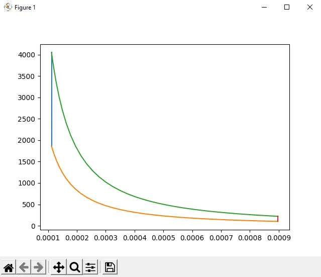
AIM: To write a program in python for the air cylinder cycle (Otto cycle), output thermal efficiency, and plot PV diagram.
OBJECTIVE:
1) To plot a PV diagram of the otto cycle using code variables in python programing, puting the proper values and command in the functioning.
2) Also to solve the thermal efficiency using apropriate formula and doing them accordingly.
THEORY:
The Otto cycle is also called the thermodynamic cycle that describes the functioning of the typical spark ignition piston engine. It is a thermodynamic cycle most found in automotive engine.
Otto cycle description of what happens to a mass of gas as it is subject to changes of pressure, temperature, volume, the addition of heat, and removal of heat. The mass of gas that is subjected to those change is called the system. The system, in this case, is defined to be fluid (gas) within the cylinder. By describing the change that take place within the system, it will also describe in the inverse, the system's effect on the environment.
The Otto cycle is constructed from:-
- Top and bottom of the loop a pair of quasi-parallel and isentropic processes (frictionless, adiabatic reversible).
- left and right sides of the loop a parallel isochoric processes.
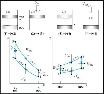
Fig 1:- Otto cycle
The processes of the otto cycle system are explain in the detail below and it would understand the coding to be written in the python program.
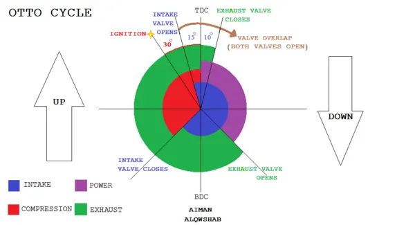
Fig 2:- Processes of the Otto cycle
Process 0-1: Intake stroke (blue shade):-
A mass of air is drawn into the cylinder or piston, the arrangement at constant pressure.
Process 1-2: compression stroke (B on diagrams):-
Is an adiabatic Isentropic compression of the charge as the piston moves from the bottom dead center to top dead center .
Process 2-3: Ignition phase (C on the diagram):-
Is a constant volume heat transfer to the working gas from the external source while the piston is at the top dead center. This process is intend to represent the ignition of the fuel-air mixture and subsequent rapid burning.
Process 3-4: Expansion stroke (D on diagram):-
Is an adiabatic (Isentropic) expansion (power stroke)
Process 4-1: Idealized heat rejection (A diagram):-
The mass of air is release into the atmosphere in a constant pressure process.
PROCEDURE:-
Coding the otto cycle:-
1) First import math for mathematical function such as sin,cos and angle. and port math plot lib for plotting the P-V diagram.
2) Giving function to the engine_kinematics (bore, stroke, connecting_rod, cr, strat_crank, end_crank):-
3) Giving value to the geometric parameter, writing code for volume parameters and stating start crak and end crank:-
- a = stroke/2
- R = connecting_ rod
- V_s = math.pi*(1/4)*pow(bore,2)*stroke
- V_c = V_s/(cr-1)
- sc = math.radians(start_crank)
- ec = math.radians(end crank)
4) Equation for calculating volume during isentropic compression and expansion process:-
v = [1+1/2.(Cr-1)[R+1 - Cosθ - √(R^2 - (sinθ) ^2)] * v_clearance
Expanding the above formulae, so that python can recognize it through inputs and give the outputs, so the formula is a divide in A, A2, and A3 and in to function range (0 to num values).
5) The initial inputs values of the intake stroke and geometric parameters are given to the process:-
- P1 = 101.35
- T1 = 500
- γ = 1.4
- T3 = 2500
- bore = 0.1
- stroke = 0.1
- connecting_rod = 0.15
- cr = 8
6) Computing the volume for v1 and v2 and for process (2-3) and :-
Pressure p2 = p1*pow(v1, gamma)/pow(v2, gamma) and for t2 =rhs = (p1*v1)/t1
t2 = (p2*v2)/rhs
7) For volume and compression process between (180 to 0), calculating the P_cpmression in volume compression by giving append to it and the th code as:-
V_compression = engine_kinematics (bore, stroke, connecting_rod, cr, 180, 0).
constant = p1*pow(v1,gamma),
P_compression = [],
for v in V_compression:-
P_compression.append(constant/pow(v,gamma)).
8) Coding for the output of P3, P4, T4, V3, and V4 and also the adiabatic expansion process where it follows the same code:
- P1 = 10135
- T1 = 500
- γ = 1.4
- T3 = 2500
- bore = 0.1
- stroke = 0.1
- connecting_rod = 0.15
- cr = 8
6) Computing the volume for v1 and v2 and for process (2-3) and
Pressure p2 = p1*pow(v1, gamma)/pow(v2, gamma) and for t2 =rhs = (p1*v1)/t1
t2 = (p2*v2)/rhs.
7) For volume and compression process between (180 to 0), calculating the P.cpmression in volume compression by giving append to it and the th code as:
V_compression = engine_kinematics (bore, stroke, connecting_rod, cr, 180, 0)
constant = p1*pow(v1,gamma)
P_compression = []
for v in V_compression:
P_compression.append(constant/pow(v,gamma)).
8) Coding for the output of P3, P4, T4, V3, and V4 and also the adiabatic expansion process where it follows the same codes:
V_expansion = engine_kinematics (bore, stroke, connecting_rod, cr, 0, 180)
constant = p3*pow(v3,gamma)
P_expansion = []
for v in V_expansion:
P_expansion.append(constant/pow(v,gamma))
9) As the otto cycle also result for the thermal efficiency which is written by the following formula in python code:
thermal_efficiency = 1 - (1/pow((connecting_rod), (gamma-1)))
print ('Thermal Efficiency of given air cylinder cycle is ', thermal_efficiency)
CODE:
#otto cycle

import math
import matplotlib.pyplot as plt

def engine_kinematics(bore, stroke, con_rod, cr, start_crank, end_crank):
	#engine_kinematics

		# geometric parameters

	a = stroke/2
	r = con_rod/a

	#volume parameters
	v_s = math.pi*(1/4)*pow(bore,2)*stroke
	v_c = v_s/(cr-1)

	sc = math.radians(start_crank)
	ec = math.radians(end_crank)

	num_values = 50

	dtheta = (ec - sc)/(num_values-1)

	v = []

	for i in range(0,num_values):
		theta = sc + i*dtheta

		term1 = 0.5*(cr-1)
		term2 = r + 1 - math.cos(theta)
		term3 = pow(r,2) - pow(math.sin(theta),2)
		term3 = pow(term3, 0.5)

		v.append((1 + term1*(term2 - term3))*v_c)

	return v

#inputs
p1 = 101.325
t1 = 500
gamma = 1.4
t3 = 2500

# geometric parameters
bore = 0.1
stroke = 0.1
con_rod = 0.15
cr = 8

#volume computation
v_s = (math.pi/4)*pow(bore,2)*stroke
v_c = v_s/(cr-1)
v1 = v_c + v_s

#state point 2
v2 = v_c

#p2v2^gamma = p1v1^gamma
p2 = p1*pow(v1,gamma)/pow(v2,gamma)

#p2v2/t2 = p1v1/t1 | rhs = p1v1/t1 | p2v2/t2 = rhs | t2 = p2v2/rhs
rhs = p1*v1/t1
t2 = p2*v2/rhs
v_compression = engine_kinematics(bore, stroke, con_rod, cr, 180, 0)

constant = p1*pow(v1,gamma)

p_compression= []

for v in v_compression:
	p_compression.append(constant/pow(v, gamma))

#state point 3
v3 = v2
#p3v3/t3 = p2v2/t2 | rhs = p2v2/t2 | p3 = rhs*t3/v3

rhs = p2*v2/t2
p3 = rhs*t3/v3

v_expansion = engine_kinematics(bore, stroke, con_rod, cr, 0, 180)

constant = p3*pow(v3,gamma)

p_expansion= []

for v in v_expansion:
	p_expansion.append(constant/pow(v, gamma))
#state point 4
v4 = v1

#p4v4^gamma = p3v3^gamma

p4 = p3*pow(v3,gamma)/pow(v4,gamma)

# p4v4/t4 = rhs
t4 = p4*v4/rhs

plt.plot([v2, v3],[p2, p3])
plt.plot(v_compression, p_compression)
plt.plot(v_expansion, p_expansion)
plt.plot([v4, v1],[p4, p1])
plt.show()
PLOT: