Week 2 Air standard Cycle

Aim: To solve an otto cycle and create a PV diagram and output the thermal efficiency of the engine.

Objectives:

1. Solve the otto cycle
2. Create a PV diagram
3. Output the thermal Efficiency of the engine

Theory:

Otto cycle is a Spark-Ignition cycle also known as Constant Volume Heat Addition cycle that describes the working of Internal Combustion engines(using gasoline as a primary fuel).

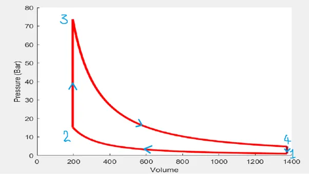
Process 1-2: Isentropic Compression Process

Process 2-3: Constant Volume Heat Addition Process

Process 3-4: Isentropic Expansion Process

Process 4-1: Constant Volume Heat Rejection Process

Calculations:

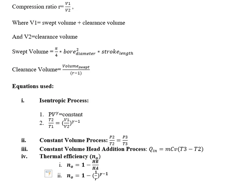
The equations to solve the otto-cycle are as below,

The code for solving the Otto cycle and generating PV diagram is as follows

#Program to solve Otto Cycle

import math
import matplotlib.pyplot as plt

def engine_kinematics(bore,stroke,con_rod,cr,start_crank,end_crank):
	a= stroke/2
	R=con_rod/a

	V_s = (math.pi)*0.25*pow(bore,2)*stroke
	V_c = V_s/(cr-1)

	sc=math.radians(start_crank)
	ec=math.radians(end_crank)

	num_values = 50


	dtheta = (ec-sc)/(num_values-1)
	V=[]

	for i in range (0, num_values):
		theta = sc + i*dtheta

		term1 = 0.5*(cr-1)
		term2 = R + 1-math.cos(theta)
		term3 = pow(R,2)-pow(math.sin(theta),2)
		term3 = pow(term3,0.5)

		V.append((1 + term1*(term2 - term3))*V_c)

	return V

#Inputs
p1 = 101325
t1=500
t3=2500
gamma=1.4

#Geometric parameters
bore =0.1
stroke = 0.15
con_rod=0.2
cr=8

#Volume Computation
V_s = (math.pi)*0.25*pow(bore,2)*stroke
V_c = V_s/(cr-1)

#State Point 1
v1=V_s + V_c

#State Point 2
v2=V_c

#p2v2^gamma = p1v1^gamma | rhs = p1v1^gamma | p2=rhs/(v2^gamma)
rhs = p1*pow(v1,gamma)
p2=rhs/(pow(v2,gamma))

#p1v1/t1 = p2v2/t2 | const = p1v1/t1 | t2=p2v2/const
const = p1*v1/t1
t2 = (p2*v2)/const
V_comp=engine_kinematics(bore,stroke,con_rod,cr,180,0)
P_comp=[]
constant = p1*pow(v1,gamma)

for v in V_comp:
	P_comp.append(constant/pow(v,gamma))

#State Point 3
v3=v2

#p2v2/t2 = p3v3/t3 | const = p2v2/t2 | p3=const*t3/v3
const = p2*v2/t2
p3=(const*t3)/v3


#State Point 4
v4=v1

#p4v4^gamma = p3v3^gamma | rhs = p3v3^gamma | p4=rhs/(v4^gamma)
rhs = p3*pow(v3,gamma)
p4=rhs/(pow(v4,gamma))
V_exp=engine_kinematics(bore,stroke,con_rod,cr,0,180)
P_exp=[]
constant = p3*pow(v3,gamma)

for v in V_exp:
	P_exp.append(constant/pow(v,gamma))


#p3v3/t3 = p4v4/t4 | t4=p4v4/const
t4 = (p4*v4)/const

thermal_efficiency = 1 - (t4-t1)/(t3-t2)
print("The Thermal effciency of the cycle is ", thermal_efficiency)

plt.plot([v2,v3],[p2,p3])
plt.plot([v4,v1],[p4,p1])
plt.plot(V_comp,P_comp)
plt.plot(V_exp,P_exp)
plt.xlabel("Volume")
plt.ylabel("Pressure")
plt.show()

Explanation:

We first define the inputs as shown for a SI Engine. Then we calculate the Swept Volume and Clearance Volume using the equation defined above. Then using all equations for each process all-state point values are calculated. To define the path between these points, I defined a function i.e. engine_kinematics which using the equation calculates the path

Result

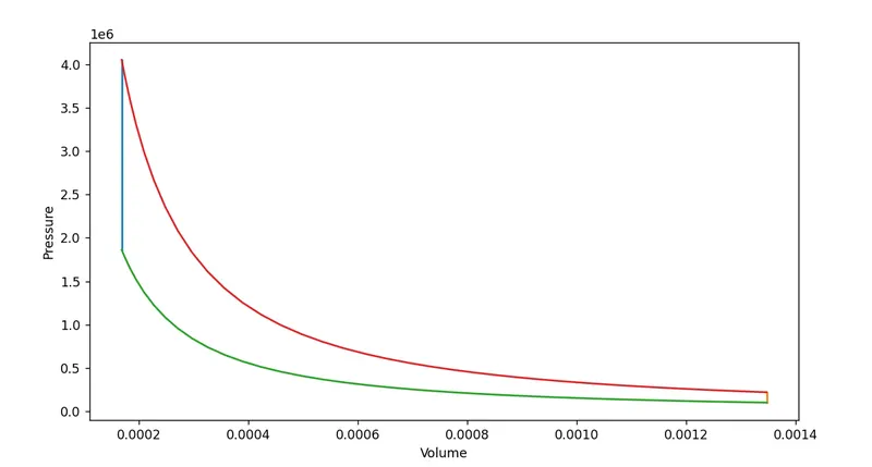
The PV plot comes out as follows

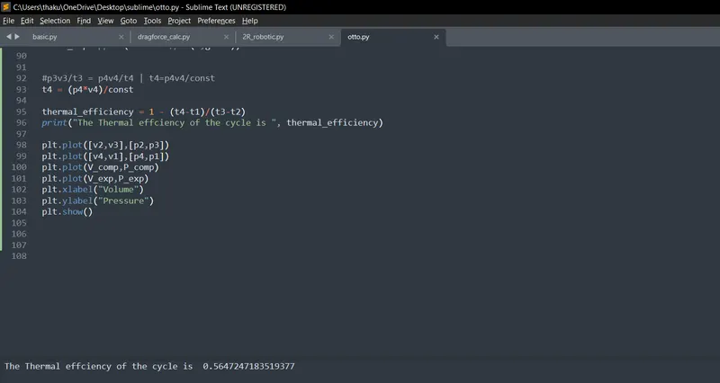
And the thermal efficiency is as follows

Conclusion

The Otto Cycle is solved and the PV Diagram is generated and the Thermal efficiency is calculated.