Week 2 Air standard Cycle

AIR STANDARD CYCLE

OBJECTIVE

• To write a program in python to create a P-V diagram of the Otto Cycle.
• To output the thermal efficiency of the engine.

PROBLEM STATEMENT

The air-standard cycle is an idealized cycle founded on the following approximations:

(1) The working fluid throughout the cycle is only air

(2) the air acts as an ideal gas

(3) combustion processes are replaced by well-defined heat addition processes

(4) the exhaust process is replaced by a heat rejection process that returns the air of the cycle to intake conditions.

Since air is assumed to be an ideal, or perfect, gas, constant values of specific heat at constant volume and pressure are frequently assumed.

The Otto cycle is an air-standard cycle which approximates the processes in petrol or diesel engines. It is based on constant volume heat addition (combustion) and heat rejection processes, and isentropic compression and expansion.

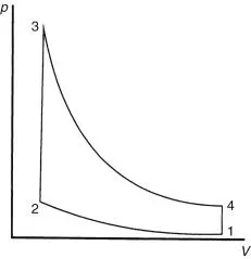
The basic Otto cycle is made up of four processes

1. Isentropic compression

2. Constant volume heat addition

3. Isentropic expansion

4. Constant volume heat rejection

The working fluid throughout the cycle is air, and this is treated as a perfect gas.The compression process 1–2 and the expansion process 3–4 are both treated as frictionless and adiabatic (without heat loss).In place of heat addition by internal combustion , phase 2–3 of the process is represented by the addition of heat from an external source, the volume remaining constant.The exhaust process is replaced by cooling at constant volume to the initial temperature.

Here we want to write a programme for plot the PV diagram of the Otto Cycle.

SOLUTION PROCEDURE

1.Python program to create P-V diagram of the Otto cycle

""" 
Programe to create PV diagram of Otto Cycle
By - ABIN K J

"""
import math
import matplotlib.pyplot as plt

#inputs
p1=101325
t1=500
t3=2300
gamma=1.4


#geometric parameters
bore=0.1
stroke=0.1
con_rod=0.15
cr=12
a=stroke/2
R=con_rod/a

#volume computation
v_s=(math.pi/4)*pow(bore,2)*stroke
v_c=v_s/(cr-1)
v1=v_c+v_s


def engine_kinematics (bore,stroke,con_rod,cr,start_crank,end_crank):
	
	sc=math.radians(start_crank)
	ec=math.radians(end_crank)

	num_values=50

	d_theta=(ec-sc)/(num_values-1)

	V=[]

	for i in range(0,num_values):
		theta=sc + i*d_theta
		term1=0.5*(cr-1)
		term2=R+1-math.cos(theta)
		term3=pow(R,2)-pow(math.sin(theta),2)
		term3=pow(term3,0.5)
		V.append((1+term1*(term2-term3))*v_c)
	return V

#state point 2
v2=v_c

#p2v2^gamma=p1v1^gamma
p2=p1*pow(v1,gamma)/pow(v2,gamma)

#p2v2/t2=p1v1/t1  
rhs=p1*v1/t1
t2=p2*v2/rhs

V_compression=engine_kinematics (bore,stroke,con_rod,cr,180,0)

constant=p1*pow(v1,gamma)
P_compression=[]

for v in V_compression:
	P_compression.append(constant/pow(v,gamma))


#state point 3
v3=v2

#p3v3/t3=p2v2/t2
rhs=p2*v2/t2
p3=rhs*t3/v3

V_expansion=engine_kinematics (bore,stroke,con_rod,cr,0,180)

constant=p3*pow(v3,gamma)
P_expansion=[]

for v in V_expansion:
	P_expansion.append(constant/pow(v,gamma))


#state point 4
v4=v1

#p4v4^gamma=p3v3^gamma
p4=p3*pow(v3,gamma)/pow(v4,gamma)

#p4v4/t4=rhs
t4=p4*v4/rhs


plt.plot(V_compression,P_compression)
plt.plot([v2,v3],[p2,p3])
plt.plot(V_expansion,P_expansion)
plt.plot([v4,v1],[p4,p1])
plt.xlabel('Volume  (V)')
plt.ylabel('Pressure (P)')

plt.show()

Code Explanations

import math : Importing math module for doing mathematical calculations.

import matplotlib.pyplot as plt : Matplotlib.pyplot is python module to plot graphs. So, here matplotlib.pyplot imported as 'plt'

#inputs are applied : Here inputs are p1=101325 (Initial pressure in pascal), t1=500 (Initial temperature in kelvin),t3=2300,
gamma=1.4

#geometric parameters : bore=0.1,stroke=0.1,con_rod=0.15 (connecting rod length),cr=12 (compression ratio) ,a=stroke/2,R=con_rod/a

v_s=(math.pi/4)*pow(bore,2)*stroke : Code for computing swept volume.

v_c=v_s/(cr-1) : Code for computing clearance volume.

v1=v_c+v_s : Initial volume formulae.

def engine_kinematics (bore,stroke,con_rod,cr,start_crank,end_crank): : Here defining a function for the calculating volume trace using the parameters bore,stroke,connecting rod length,starting cran angle,ending crank angle.

sc=math.radians(start_crank) : Code for converting input starting crank angle from degree to radians.

ec=math.radians(end_crank) : Code for converting input ending crank angle from degree to radians.

num_values=50 : Assigning the range value for creating 'for' loop.

d_theta=(ec-sc)/(num_values-1) : Code for calculating crank angle gape to compute theta values.

V=[] : Empty array for asssigning calculated volume trace.

for i in range(0,num_values): :Creating the 'for' loop for calculating theta values.

theta=sc + i*d_theta : Formula for calculating theta values depending on 'i' value and 'd_theta'value.

term1=0.5*(cr-1) : Calculating the each splitted term in the equation of volume ratio formulae.

term2=R+1-math.cos(theta) : Calculating the second term in volume ratio formulae.

term3=pow(R,2)-pow(math.sin(theta),2) : Calculating the third term in volume ratio formulae.

term3=pow(term3,0.5) : Calculating equation terms.

V.append((1+term1*(term2-term3))*v_c) : Appending the calculated volume trace in the empty array.

return V : Code for returning the value in V.

v2=v_c : State point 2 volume condition.

p2=p1*pow(v1,gamma)/pow(v2,gamma) : Formulae for pressure at state point 2.

rhs=p1*v1/t1 : Calculating t2 from the p2v2/t2=p1v1/t1 equation. Assigning rhs value for making calculatoin simple.

t2=p2*v2/rhs : Finding temperature at state point 2.

V_compression=engine_kinematics (bore,stroke,con_rod,cr,180,0) : Calling the engine kinematics function and storing values of calclulated volume trace for starting crank angle 180 and ending carnk angle 0.These values get stored in V_compression array.

constant=p1*pow(v1,gamma) : Finding Constant value for calculating compression pressure.

P_compression=[] : Creating an empty array for storing calculated values of compression pressure.

for v in V_compression: : Creating ' for ' loop for compression pressure calculation on each values of v in V_compression array.

P_compression.append(constant/pow(v,gamma)) :Code for calculating compression pressure and appending it on the P_compresssion empty array.

v3=v2 : Volume condition at state point 3.

rhs=p2*v2/t2 : Calculating p3 from the p3v3/t3=p2v2/t2 equation. Assigning rhs value for making calculatoin simple.

p3=rhs*t3/v3 : Finding pressure at state point 3.

V_expansion=engine_kinematics (bore,stroke,con_rod,cr,0,180) :Calling the engine kinematics function and storing values of calclulated volume trace for starting crank angle 0 and ending carnk angle 180.These values get stored in V_expansion array.

constant=p3*pow(v3,gamma) : Finding Constant value for calculating expansion pressure.

P_expansion=[] : Creating an empty array for storing calculated values of expansion pressure.

for v in V_expansion: : Creating ' for ' loop for expansion pressure calculation on each values of v in V_expansion array.

P_expansion.append(constant/pow(v,gamma)) : Code for calculating expansion pressure and appending it on the P_expansion empty array.

v4=v1 : Volume condition at state point 4.

p4=p3*pow(v3,gamma)/pow(v4,gamma) : Calculating pressure at stae point 4.

t4=p4*v4/rhs : Calculating temperature at state point 4.

plt.plot(V_compression,P_compression) : Code for plotting Isentropic compression process.

plt.plot([v2,v3],[p2,p3]) : Code for plotting constant volume heat addition process.

plt.plot(V_expansion,P_expansion) : Code for plotting Isentropic expansion process.

plt.plot([v4,v1],[p4,p1]) : Code for plotting constant volume heat rejection.

plt.xlabel( 'Volume (V) ') : Code for label the 'x axis' as 'Volume (V)'

plt.ylabel( 'Pressure (P) ') : Code for label the 'y axis' as 'Pressure (P)'

plt.show() : Code for showing the plotted graph.

2.Programme to output the thermal efficiency of the engine.

"""
Programe to output the Thermal efficiency of Engine
By ABIN K J

"""

import math

#inputs
cr=12
gamma=1.4

#Thermal efficiency = 1-(1/(cr)^(gamma-1))
term1=pow(cr,(gamma-1))
term2=1/term1
Thermal_Efficiency = (1-term2)*100

Thermal_Efficiency_percentage =round(Thermal_Efficiency,2)


print(Thermal_Efficiency_percentage)

Code Explanations

import math : Importing math module for doing mathematical calculations.

#inputs are applied : Here inputs are compression ratio (cr= 12),gamma=1.4

#Therma efficiency = 1-(1/(cr)^(gamma-1)) : Formulae of thermal efficiency for reference.

term1=pow(cr,(gamma-1)) : Calculating first term in the given formula.

term2=1/term1 : Calculating term 2.

Thermal_Efficiency = (1-term2)*100 :Calculating thermal efficiency and it is multiplied with 100 to get the value in percentage.

Thermal_Efficiency_percentage =round(Thermal_Efficiency,2) : Here we use the 'round' function in python , to round the value upto 2 decimal points. And the result value is named as 'Thermal_Efficiency_percentage'.

print(Thermal_Efficiency_percentage) : Using the print command to output the thermal efficiency of the engine.

RESULTS

1.P-V diagram of Otto cycle

Thus the Pressure - Volume Diagram of Otto Cycle has been plotted using Python programing.

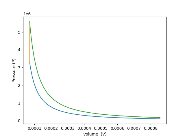
This is the plot of Otto Cycle, This plot is also attached in the answer box given below.

2.Thermal Efficiency of the Engine

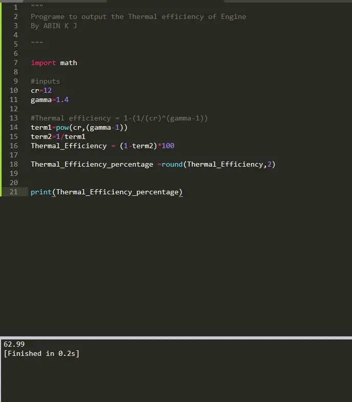
Thus the Programme for output the thermal efficiency of the engine is written and printed.

Output

Thermal efficiency = 62.99

EXPLANATION OF RESULTS

1.P-V diagram of Otto cycle

Here , the each process in the otto cycle had plotted in different stroke colours.

• Isentropic Compression = It is plotted here in blue colour. Graph is curved shape.
• Constant Volume heat addition = It is plotted here in orange colour.It is a straight line.
• Isentropic Expansion = It is plotted here in green colour. Graph is curved shape.
• Constant Volume heat rejection = It is plotted here in red colour.It is a straight line.

2.Thermal Efficiency of the Engine

Here the thermal efficiency of engine is calculated and is converted to percentage. The final value is rounded up to 'two' decimals.

Thermal Efficiency = 62.99%