2R ROBOTIC ARM SIMULATOR

2R ROBOTIC ARM SIMULATOR

OBJECTIVE

• To write a program in python to simulate the forward kinematics of a 2R Robotic Arm.
• To create an animation file of the plot.

PROBLEM STATEMENT

Forward kinematics refers to the use of the kinematic equations of a robot to compute the position of the end-effector from specified values for the joint parameters.The end-effector is the working end of a robotic arm. Different parameters are taken to account for calculation of the end effector position. The end-effector attached to the end of link 2 to perform various tasks.

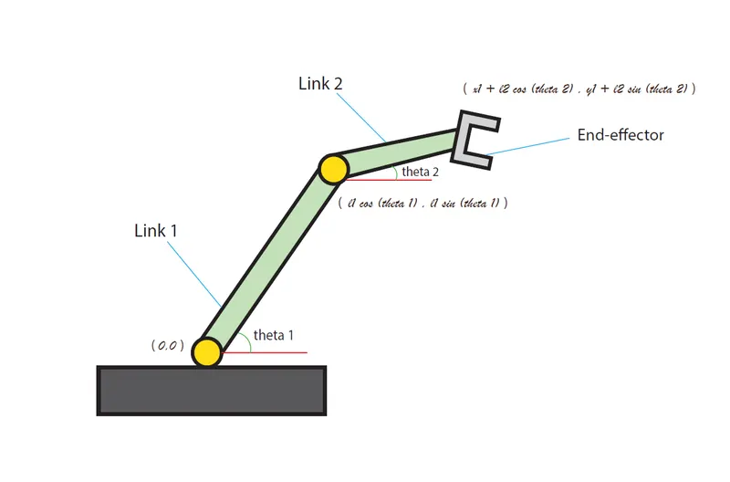
Here ,

l1 = Link 1 (Length of Link 1)

l2 = Link 2 (Length of Link 2)

theta 1 = Angle between link 1 and horizontal axis.

theta 2 = Angle between link 2 and horizontal axis.

Positional coordinates are ,

Base of link 1 = (0,0) fixed in origin.

End of link 1 or Base of link 2 = ( l1 cos (theta 1) , l1 sin (theta 1) )

End of link 2 = ( x1 + l2 cos (theta 2) , y1 + l2 sin (theta 2) )

The plots are made about ,

[ (x0 , x1) , (y0 , y1) ] = For plotting Link 1

[ (x1 , x2) , (y1 , y2) ] = For plotting link 2

Based on these datas we can trace the positions of robotic arm for each theta value.

SOLUTION PROCEDURE

1. Python to simulate the forward kinematics of a 2R Robotic Arm

"""
Programe to Animate 
- Forward Kinematics of a 2R Robotic arm
  Done by ABIN K J

"""

import math
import matplotlib.pyplot as plt

#inputs
l1=1
l2=0.5

x0=0
y0=0


n_theta=10
theta_start=0
theta_end=math.pi/2

theta1=[]
theta2=[]

for i in range(0,n_theta):
	tmp=theta_start +  i*(theta_end-theta_start)/(n_theta-1)
	theta1.append(tmp)
	theta2.append(tmp)


ct=1
for t1 in theta1:
	for t2 in theta2:

		#Link1-Link2 Connector
		x1= l1*math.cos(t1)
		y1= l1*math.sin(t1)

		#Coordinates of the manipulator
		x2= x1 + l2*math.cos(t2)
		y2= y1 + l2*math.sin(t2)

		filename = str(ct) + '.png'
		ct=ct+1

		plt.figure()
		plt.plot([x0,x1],[y0,y1])
		plt.plot([x1,x2],[y1,y2])
		plt.xlim([0,2])
		plt.ylim([0,2])
		plt.savefig(filename)

Code Explanations

import math : math module is used for doing mathematical calculations.

import matplotlib.pyplot as plt : matplotlib.pyplot is python module to plot graphs. So, here matplotlib.pyplot imported as 'plt'

inputs are applied : Here input values are applied,Length of arm 1 (l1) =1 , Length of arm 2 (l2)=0.5

x0=0 : Base of first arm fixed in origin. x0=0

y0=0 : Base of first arm fixed in origin. y0=0

n_theta=10 : Condition for assigning ten values for theta.

theta_start=0 : Theta values are assigning between 0 to pi/2. So starting angle for the range of theta values.

theta_end=math.pi/2 : Ending value for the range of theta is 90 degree, so using math module the pi/2 value is assigned.

theta1=[] : An empty array created for storing the ten theta1 values.

theta2=[] : Another empty array created for storing the ten theta2 values.

for i in range(0,n_theta): : Creating for loop for assigning then theta values ,in the range of 0 to 10.

tmp=theta_start + i*(theta_end-theta_start)/(n_theta-1) : Creating a function tmp , for calculating theta values between the range.

theta1.append(tmp) : Appending each value of theta calculated using tmp in theta1 empty array.

theta2.append(tmp) : Since theta values are same , tmp function again used to append theta values in theta2 empty array.

ct=1 : Creating a counter for naming the files in a serial number order.

fot t1 in theta1: : Creating a for loop , for making calculations associated with theta1 array.

for t2 in theta2: : Creating an another for loop inside the first one , for making calculations on every theta 2 values associated with each theta1 values.

x1= l1*math.cos(t1) : Formula for calculating x1 coordinate for each theta1(t1) value.

y1= l1*math.sin(t1) : Formula for calculating y1 coordinate for each theta1(t1) value.

x2= x1 + l2*math.cos(t2) : Formula for calculating x2 coordinate for each theta2(t2) value.

y2= y1 + l2*math.sin(t2) : Formula for calculating y2 coordinate for each theta2(t2) value.

filename = str(ct) + '.png' : Code for saving each polt in serial number order using 'ct' variable , with '.png' extension.

ct=ct+1 : Counter variable function to get increasing number order.

plt.figure() : Code for plot each position of arm using matplot module.

plt.plot([x0,x1],[y0,y1]) : Code for potting first link position.

plt.plot([x1,x2],[y1,y2]) : Code for potting second link position.

plt.xlim([0,2]) : Code for fixing the x axis limit.

plt.ylim([0,2]) : Code for fixing the y axis limit.

plt.savefig(filename) : Command for saving each plot in prepared filename.

RESULTS

The simulation gif is created by using image magick software , and the animation video is uploaded in youtube.

Here is the youtube link of uploaded video

Link - https://youtu.be/IlWQ_2qK4Iw

EXPLANATION OF RESULTS

The position of Link 2 is varies for every theta2 values repetitively according to different position of link 1. That is for each and every position of link1 , link 2 will aquire every possible position. This positional changes are used for different applications, because end-effector can able to reach any position.