Week 3 - Solving second order ODEs
SOLVING SECOND ORDER ODEs
OBJECTIVE
- To write a python program that solve the following ODE. This ODE represents the equation of motion of a simple pendulum with damping
- To write a program in Python that will simulate the pendulum motion.
PROBLEM STATEMENT
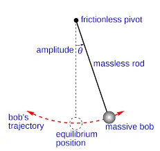
In Engineering, ODE is used to describe the transient behavior of a system. A simple example is a pendulum
The way the pendulum moves depends on the Newtons second law. When this law is written down, we get a second order Ordinary Differential Equation that describes the position of the "ball" w.r.t time.
Similarly, there are hundreds of ODEs that describe key phenomena and if you have the ability to solve these equations then you will be able to simulate any of theses systems.
This ODE represents the equation of motion of a simple pendulum with damping
In the above equation,
g = gravity in m/s2,
L = length of the pendulum in m,
m = mass of the ball in kg,
b=damping coefficient.
Here,
L=1 metre,
m=1 kg,
b=0.05.
g=9.81 m/s2.
SOLUTION PROCEDURE
1.Python programme to solve the second order ODE.
"""
1-Code for solving second order ODE
by-ABIN K J

"""
import numpy as np
from scipy.integrate import odeint
import matplotlib.pyplot as plt
import math

#function that returns dz/dt
def model(theta,t,b,g,l,m):
	theta1=theta[0]
	theta2=theta[1]
	dtheta1_dt=theta2
	dtheta2_dt=-(b/m)*theta2 - (g/l)*math.sin(theta1)
	dtheta_dt=[dtheta1_dt,dtheta2_dt]
	return dtheta_dt
b=0.02
g=9.81
l=1
m=0.1

#initial condition
theta_0=[math.pi/2,0]

#time points
t=np.linspace(0,10,150)

#solve ODE
theta=odeint(model,theta_0,t,args=(b,g,l,m))

plt.plot(t,theta[:,0],'b-',label=r'$frac{dtheta1}{dt}=theta2$')
plt.plot(t,theta[:,1],'r--',label=r'$frac{dtheta2}{dt}=-frac{b}{m}theta2-frac{g}{L}sintheta1$')
plt.xlabel('Time')
plt.ylabel('Plot')
plt.legend(loc='best')
plt.show()
Code Explanations
import numpy as np : Importing numpy module to doing numerical calculations.
from scipy.integrate import odeint : Importing odient module from scipy to solving second order ODE.
import matplotlib.pyplot as plt : Matplotlib.pyplot is python module to plot graphs. So, here matplotlib.pyplot imported as 'plt'
import math : Importing math module for doing mathematical calculations.
def model(theta,t,b,g,l,m): : Definig the function to solve ODE.
theta1=theta[0] : Assigning theta1 value to the first column of theta array
theta2=theta[1] : Assigning theta2 value to the second column of theta array
dtheta1_dt=theta2 : Equating theta2 value to dtheta1_dt value.This is the first ODE
dtheta2_dt=-(b/m)*theta2 - (g/l)*math.sin(theta1) : Defining second ODE
dtheta_dt=[dtheta1_dt,dtheta2_dt] : Compined array of first and second ODE.
return dtheta_dt : Returning dtheta_dt value.
b=0.02 : Damping coefficient value.
g=9.81 : Acceleration due to gravity value.
l=1 : Length of the pendulum.
m=0.1 : Mass of the bob.
theta_0=[math.pi/2,0] : Initial conditions , [Displacement,Initial velocity]
t=np.linspace(0,10,150) : Time values. Using linespace module to split 150 equal values of theta between 0 and 10.
theta=odeint(model,theta_0,t,args=(b,g,l,m)) : Code for solving ODE using odeint module.It integrate defined functions with respect to given time limit.
plt.plot(t,theta[:,0],'b-',label=r'$frac{dtheta1}{dt}=theta2$') : Code plotting displacement graph. It plots the first column values of theta array. Writing code for legend in graph.
plt.plot(t,theta[:,1],'r--',label=r'$frac{dtheta2}{dt}=-frac{b}{m}theta2-frac{g}{L}sintheta1$') : Code plotting velocity graph. It plots the second column values of theta array. Writing code for legend in graph.
plt.xlabel('Time') : Code or labeling x axis as 'Time'
plt.ylabel('Plot') : Code or labeling y axis as 'Plot'
plt.legend(loc='best') : Code for plcaing legent labels to the best free position in graph.
plt.show() : Code for showing the plotted graph.
2.Python programme to animate pendulum motion.
"""
2- Code for pendulum animation
by-ABIN K J
"""

import numpy as np
from scipy.integrate import odeint
import matplotlib.pyplot as plt
import math


#function that returns dz/dt
def model(theta,t,b,g,l,m):
	theta1=theta[0]
	theta2=theta[1]
	dtheta1_dt=theta2
	dtheta2_dt=-(b/m)*theta2 -(g/l)*math.sin(theta1)
	dtheta_dt=[dtheta1_dt,dtheta2_dt]
	return dtheta_dt
b=0.05
g=9.81
l=1
m=1

#initial condition

theta_0=[0,3]

#time points
t=np.linspace(0,20,150)

#solve ODE
theta=odeint(model,theta_0,t,args=(b,g,l,m))

#animation
ct = 1

for i in theta[:,0]:
	x = (l*math.sin(i))
	y = (-l*math.cos(i))
	filename = 'test%05d.png' % ct
	ct = ct +1
	plt.figure()
	plt.plot([-1,1],[0,0],"black",linewidth=10)
	plt.plot([0,x],[0,y],"red")
	plt.plot(x,y,'o',markersize = 20)
	plt.xlim([-1.5,1.5])
	plt.ylim([-1.5,1.0])
	plt.savefig(filename)
Code Explanations
import numpy as np : Importing numpy module to doing numerical calculations.
from scipy.integrate import odeint : Importing odient module from scipy to solving second order ODE.
import matplotlib.pyplot as plt : Matplotlib.pyplot is python module to plot graphs. So, here matplotlib.pyplot imported as 'plt'
import math : Importing math module for doing mathematical calculations.
def model(theta,t,b,g,l,m): : Definig the function to solve ODE.
theta1=theta[0] : Assigning theta1 value to the first column of theta array
theta2=theta[1] : Assigning theta2 value to the second column of theta array
dtheta1_dt=theta2 : Equating theta2 value to dtheta1_dt value.This is the first ODE
dtheta2_dt=-(b/m)*theta2 - (g/l)*math.sin(theta1) : Defining second ODE
dtheta_dt=[dtheta1_dt,dtheta2_dt] : Compined array of first and second ODE.
return dtheta_dt : Returning dtheta_dt value.
b=0.05 : Damping coefficient value.
g=9.81 : Acceleration due to gravity value.
l=1 : Length of the pendulum.
m=1 : Mass of the bob.
theta_0=[0,3] : Initial conditions , [Displacement,Initial velocity]
t=np.linspace(0,20,150) : Time values. Using linespace module to split 150 equal values of theta between 0 and 10.
theta=odeint(model,theta_0,t,args=(b,g,l,m)) : Code for solving ODE using odeint module.It integrate defined functions with respect to given time limit.
ct = 1 : Defining counter.
for i in theta[:,0]: : Creating for loop for each value of displacement from theta array.
x = (l*math.sin(i)) : Code for tracing x coordinte.
y = (-l*math.cos(i)) : Code for tracing y coordinte.
filename = 'test%05d.png' % ct : Code for saving each plotted graph , naming 'test' , a five digit serial number will also added according to the counter value while looping through.
ct = ct +1 : Counter value reassigned as 'ct = ct+1'
plt.figure() : Code for plotting figures.
plt.plot([-1,1],[0,0],"black",
plt.plot([0,x],[0,y],"red") : Code for plotting pendulum.
plt.plot(x,y,'o',markersize = 20) : Code for plotting bob.
plt.xlim([-1.5,1.5]) : Assigning limits for x axis.
plt.ylim([-1.5,1.0]) : Assigning limits for x axis.
plt.savefig(filename) : Code for saving each plot using defined file name.
RESULT
1.Solving ODE.
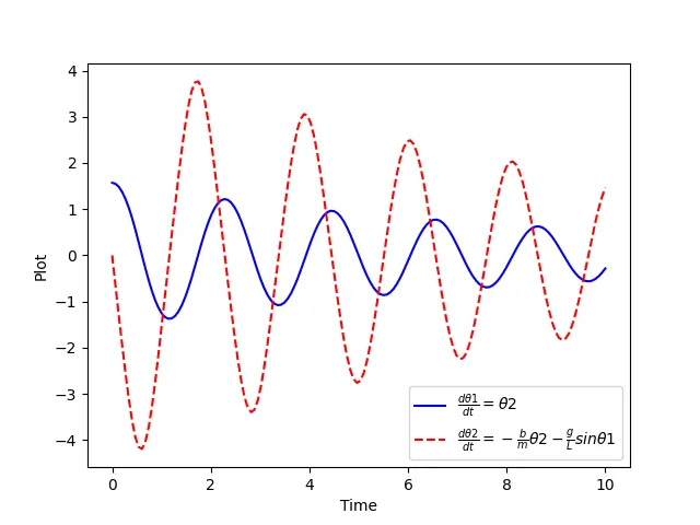
The given graph represents the Position,Velocity-Time plot of the simple pendulum.
2.Pendulum Animation
The simulation gif is created by using image magick software , and the animation video is uploaded in youtube.
Here is the youtube link of uploaded video
YouTube Link - https://youtu.be/P4_GzffvzRI
(A mp4 video also uploaded in answer box)
EXPLANATION OF RESULTS
1.Simple pendulum graph
The given second order ODE is solved using python programming , and this soulution is used to plot the Position, Velocity - Time graph of the simple pendulum.
The solved equations are added in graph and they are made to easily identify the plot.
2.Pendulum Animation
Simple pendulum is animated by combining different plots of pendulum at different time periods.Thus the pendulum is created as per the given conditions.
ERRORS FACED
The error i was faced while programming is typing mistake while defining second ODE. It made an unexpected result plot.
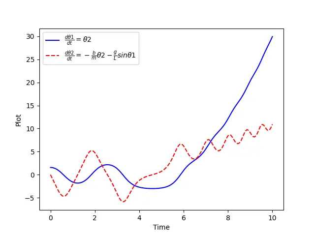
ERROR SOLUTION
Error in Code
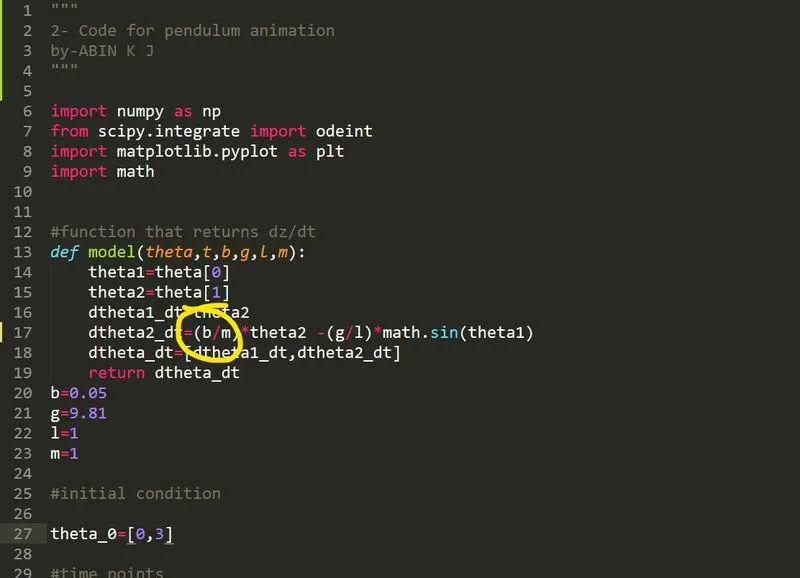
Here i missed a negative sign in line number 17.
Error in code : dtheta2_dt= (b/m)*theta2 -(g/l)*math.sin(theta1)
Corrected Code

Error is corrected here : dtheta2_dt= -(b/m)*theta2 -(g/l)*math.sin(theta1)
Negative sign added before (b/m) term