Week 2 Air standard Cycle

Aim: To write a code to simulate an Otto cycle and plot its Pv diagram

Governing equation:

• Thermal efficiency of an engine can be simply given by the fraction of energy added by heat that is converted into net work output.

For an engine working on Otto cycle (like petrol engine),the thermal efficiency is given by the following equation:

`eta th=1-1/(r^(gamma-1)`

where `etath`,`r` and `gamma ‘represent respectively the thermal efficiency the compression ratio and the adiabatic constant of the working fluid.

• `P*V^gamma=c` is an equation related to isentropic processes, where `P` and `V` stand respectively for pressure and volume and `gamma` the adiabatic index .For an isentropic process going from state 1(`P1,V1`) to state 2(`P2,V2`) , `P1*V1^gamma=P2*V2^gamma=c`

The swept volume `Vswept` and the clearance volume `V_comp` are given by the following equations:`Vswept=(pi/4)*b^2*stroke` where b is the bore and `V_comp= V_swept//(Cr-1)`

Objectives:

• Write a program in Python to plot the PV diagram of an Otto cycle
• Output the thermal efficiency of the engine (working on Otto cycle)

Theory:

Otto cycle is an idealised thermodynamic cycle made up of 4 internally reversible processes and which is used in SI engines (Spark Ignition) engines.

These four processes are:

• Isentropic compression
• Isochoric heat addition
• Isentropic expansion (power stroke)
• Constant volume heat rejection

The P-V diagram of this cycle is shown in the output of the code shown in this report.

Coding:

The program written in this project to simulate Otto cycle is shown below.

To plot the isentropic compression and expansion processes paths,a function named 'Engine_kinematics' has been written and called inside the main program.

• Function

def Engine_kinematics(bore,stroke,con_rod,Cr,start_crank_angle,end_crank_angle):
	#Engine_kinematics
	import math
	#Geometric parameters
	#Crank pin radius
	a=stroke/2
	R=con_rod/a
	#Volume parameters
	V_swept=(math.pi/4)*pow(bore,2)*stroke
	V_comp=V_swept/(Cr-1)
	V=[]
	#Converting angles in radians

	s_c=math.radians(start_crank_angle)
	e_c=math.radians(end_crank_angle)
	num_values=100
	dtheta=(e_c-s_c)/(num_values-1)
	for i in range(0,num_values):
		theta=s_c+i*(dtheta)
		
		term1=0.5*(Cr-1)
		term2=R+1-math.cos(theta)
		term3= pow(pow(R,2)-pow(math.sin(theta),2),0.5)

		V.append(V_comp*(1+term1*(term2-term3)))
	return V

• Main code

#Otto cycle simulaor
import math
import matplotlib.pyplot as plt


def Engine_kinematics(bore,stroke,con_rod,Cr,start_crank_angle,end_crank_angle):
	#Engine_kinematics
	import math
	#Geometric parameters
	#Crank pin radius
	a=stroke/2
	R=con_rod/a
	#Volume parameters
	V_swept=(math.pi/4)*pow(bore,2)*stroke
	V_comp=V_swept/(Cr-1)
	V=[]
	#Converting angles in radians

	s_c=math.radians(start_crank_angle)
	e_c=math.radians(end_crank_angle)
	num_values=100
	dtheta=(e_c-s_c)/(num_values-1)
	for i in range(0,num_values):
		theta=s_c+i*(dtheta)
		
		term1=0.5*(Cr-1)
		term2=R+1-math.cos(theta)
		term3= pow(pow(R,2)-pow(math.sin(theta),2),0.5)

		V.append(V_comp*(1+term1*(term2-term3)))
	return V

  

#Inputs
T1=500
P1=101325

#Gemetric parameters
bore=0.1
stroke=0.1
con_rod=0.15
Cr=12
T3=2300
gamma=1.4
#Volume computation
V_swept=(math.pi/4)*pow(bore,2)*stroke
V_comp=V_swept/(Cr-1)
V1=V_swept+V_comp

#state point 2
V2=V_comp
#p1v1^gamma=p2v2^gamma
P2=P1*pow(V1,gamma)/pow(V2,gamma)
#P1V1/T1=P2V2/T2
T2=P2*V2*T1/(P1*V1)
cst=P1*pow(V1,gamma)
V_compression=Engine_kinematics(bore,stroke,con_rod,Cr,180,0)
P_compression=[]
for v in V_compression:
	P_compression.append(cst/pow(v,gamma))



#State point 3
V3=V2
#P2V2/T2=P3V3/T3
P3=P2*V2*T3/(V3*T2)
cst=P3*pow(V3,gamma)
V_Expansion=Engine_kinematics(bore,stroke,con_rod,Cr,0,180)
P_Expansion=[]
for k in V_Expansion:
	P_Expansion.append(cst/pow(k,gamma))
	
#State point 4
V4=V1
#P3V3^gamma=P4V4^gamma
P4=P3*pow(V3,gamma)/pow(V4,gamma)

#P4V4/T4=P3V3/T3
T4=P4*V4*T3/(P3*V3)

#Plotting constant volume heat addition state curve
plt.plot([V2,V3],[P2,P3])

	#Plotting isentropic compression

plt.plot(V_compression,P_compression)
#Plotting isentropic expansion
plt.plot(V_Expansion,P_Expansion)

#Plotting constant volume heat rejection state curve

plt.plot([V4,V1],[P4,P1])
#Labelling x-axis
plt.xlabel('Volume')
#Labelling y-axis 
plt.ylabel('Pressure')
plt.show()
 #Calculation of thermal efficiency of Otto Cycle
n_th=(1-pow((1/Cr),gamma-1))*100
print('The thermal efficiency of the engine working on this Otto cycle is: ',n_th,'%')

Explanation of the Code:

• First of all, "math "module is imported as mathematical tasks with trigonometric functions have been performed in the program.

• import math

• Secondly "matplotlib” module has been also imported to perform plotting tasks in the code.

• import matplotlib.pyplot as plt

• And then, the inputs :the adiabatic index "gamma", the temperature after the heat addition "T3",the state variables at state 1 before the compression process(P1,T1) and the engine geometric parameters (bore, stroke, connecting rod length "con_rod "and the compression ratio "Cr" are declared.
• Further, the swept volume and the clearance volume of the engine are calculated using their formulae stated in the "governing equations" section of the report.
• With these calculations, volumes before compression V1 and after compression V2 are computed.
• After, the pressure after compression process P2 is computed using gas isentropic process equation. The isochoric boundary condition is used for determining the pressure P3(after the constant volume heat addition) and the pressure after power stroke is computed with similar method as P2.
• The volumes after heat addition and before heat addition are equal(V2=V3=V_comp), same as the volumes before and after heat rejection (V1=V4=V_comp+V_swept).
• Once all the state variables are declared, a function named Engine_kinematics is written to show how the volume changes with the crank angle as the piston moves from BDC to TDC.
• This function is further used in plotting the paths of the two isentropic processes of the cycles. Isochoric processes are then also plotted as straight lines with the help of coordinates of state points previously computed.
• The graph is labelled and and displayed.
• Finally, the thermal efficiency of this otto cycle is computed using its formula.

Output:

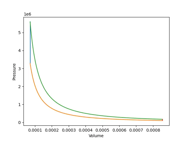
Results:

Hence, the P-v diagram of the Otto cycle has been plotted and its four processes can be clearly seen.

The thermal efficiency is also computed and displayed as shown in the output .