Week 4.1 - Genetic Algorithm

Aim: To write a code in MATLAB to optimize the stalagmite function and find the global maxima of the function.

Objectives:

• Clearly explain the concept of genetic algorithm and its syntax in MATLAB.
• Plot graphs for all 3 studies and for F maximum vs number of iterations.

Theory:

• Concept of Genetic algorithm:

Genetic algorithm (ga) is one of the reliable optimization techniques used in numerous areas nowadays.

Developed by Golderd and inspired by Darwin's theory of evolution(Only the fittest species will survive),the particularity of genetic algorithm is the fact that it is based on the principles of genetics and natural selection.

It is important to recall that in genetic algorithm, we initially have a pool of possible solutions a a given problem.

These candidate solutions will,like in natural genetics,undergo recombination and mutation to produce new individuals,and the process is repeated for a number of generations.

Each new individual(candidate solution) is alloted a fitness value and the fitter individuals are given a higher chance to recombine and yield new individuals with a higher fitness value.

As long as the process of recombination of fitter individuals will be repeated all over the successive generations,fitter "children" will be produced and hence , an optimal solution to the given problem will be obtained.

Genetic algorithm can be applied to solve problems that are not well suited for standard optimization algorithms,including problems in which the objective function is discontinuous,nondifferentiable,stochastic or highly nonlinear.

• Basic terminology related to Genetic algorithm:

• Population:it is the subset of all possible solutions of a given problem.
• Chromosome: It is one solution among the population.
• Gene: It is one element position of a chromosome.
• Allele: It is the value that a gene takes for a particular chromosome.
• Fitness function:It is the function which takes the solution as input and produces the suitability of the solution as output.
• Genotype: It is the population in the computation space(encoded population),represented in a way which can be easily understood and manipulated by a computing system.
• Phenotype:It is the population in the actual real world solution space .
• Genetic operators:These alter the genetic composition of the offspring;these include mutation,crossover,...

• Syntax of a genetic algorithm:

The syntax of genetic algorithm (ga)depends upon the objective of the function and the constraints under which it is subjected.

Below are the different syntaxes of ga:

• x = ga(fun,nvars) finds a local unconstrained minimum, x, to the objective function, fun. nvars is the dimension (number of design variables) of fun.

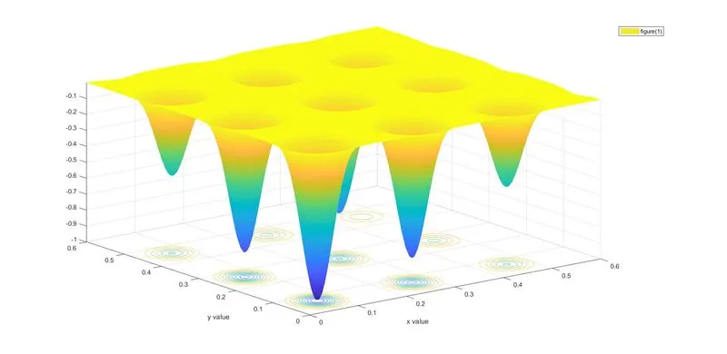
• Code: In this project ,the given stalagmite function shown in the above image is coded and willbe further called in the main code.
• Function:

function f=stalagmite(input_vector)
x=input_vector(1);
y=input_vector(2);
a=(sin(5.1*pi*x+0.5))^6;
b=(sin(5.1*pi*y+0.5))^6;
c=exp(-4*log(2)*((x-0.0667)^2/0.64));
d=exp(-4*log(2)*((y-0.0667)^2/0.64));
f=-1*a*b*c*d;
end

• Main code:

clear all
close all
clc
%stalagmite function_Genetic algorithm
%Creating our search sapce

x=linspace(0,0.6,150);
y=linspace(0,0.6,150);
num_cases=50;
%Creating a 2d mesh
[xx,yy]= meshgrid(x,y);
%evaluating the stalagmite function
for i=1:length(xx)
    for  j=1:length(yy)
       
        input_vector(1)=xx(i,j);
        input_vector(2)=yy(i,j);
        f(i,j)= stalagmite(input_vector);
    end
end
figure(1)
surfc(xx,yy,f)
xlabel('x value')
ylabel('y value')
shading interp
% [inputs,fval]=ga(@stalagmite,2)
%Study_1_Statistical behaviour
tic
for i=1:num_cases
[inputs,fopt(i)]=ga(@stalagmite,2);
xopt(i)=inputs(1);
yopt(i)=inputs(2);
end
study1_time=toc
figure(2)
subplot(2,1,1)
surfc(x,y,f)
hold on 
shading interp
title('Unbounded inputs')
plot3(xopt,yopt,fopt,'marker','o','markersize',5,'markerfacecolor','r')
subplot(2,1,2) 
plot(fopt)
xlabel('iterations')
ylabel('function minimum')

 %Study-2:statistical behaviour with upper and lower bounds
tic
for i=1:num_cases
[inputs_b,fopt2(i)]=ga(@stalagmite,2,[],[],[],[],[0;0],[1;1]);
xopt2(i)=inputs_b(1);
yopt2(i)=inputs_b(2);
end
study2_time=toc
figure(3)
subplot(2,1,1)
surfc(x,y,f)
hold on 
shading interp
title('Bounded inputs')
plot3(xopt2,yopt2,fopt2,'marker','o','markersize',5,'markerfacecolor','r')
subplot(2,1,2)
plot(fopt2)
xlabel('iterations')
ylabel('function minimum')
%Study_3:increasing the Population size
options =optimoptions('ga');
options =optimoptions(options,'populationsize',300)
tic
for i=1:num_cases
[inputs_c,fopt3(i)]=ga(@stalagmite,2,[],[],[],[],[0;0],[1;1],[],[],options);
xopt3(i)=inputs_c(1);
yopt3(i)=inputs_c(2);
end
study3_time=toc
figure(4)
subplot(2,1,1)
surfc(x,y,f)
hold on
shading interp
title('Bounded inputs with increased population')
plot3(xopt3,yopt3,fopt3,'marker','o','markersize',5,'markerfacecolor','r')
subplot(2,1,2)
plot(fopt3)
xlabel('iterations')
ylabel('function minimum')

• Explanation of the code:

• First of all, for starting a code in MATLAB, it’s highly recommended to use these three basics commands namely:"clc" to clear the command window, “clear all "to completely clear the workspace and ,''close all" to close all the graphs.

clear all
close all
clc

• Declaration of the two linspace vectors(x and y ) and the number of iterations num_cases.

  x=linspace(0,0.6,150);
  y=linspace(0,0.6,150);
  num_cases=50;​

• Creating our search space with the the messgrig [xx,yy] of two linspace vectors x and y

[xx,yy]= meshgrid(x,y);

• Evaluating the stalagmite function with the help of for loop.

%evaluating the stalagmite function
for i=1:length(xx)
    for  j=1:length(yy)
       
        input_vector(1)=xx(i,j);
        input_vector(2)=yy(i,j);
        f(i,j)= stalagmite(input_vector);
    end
end

• Plotting the surf of Stalagmite function(provided in the course)

surfc(xx,yy,f)

• Labelling the axes and shading the surf with the help of "shading interp " command.

xlabel('x value')
ylabel('y value')
shading interp
legend('figure(1)')

• tic toc command is used to measure the elapsed time.

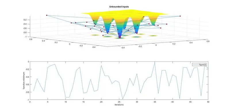
The Study-1 section of the code evaluates the statistical behaviour of stalagmite function with unbounded inputs

• Here a for loop is used to evaluates the stalagmite function with bounded inputs all over the 50 iterations.
• Then,the both the surf of the "bounded inputs stalagmite function" and the "function minimum vs number of iterations" are plotted in the same figure(2) using subplot command.

tic
for i=1:num_cases
[inputs,fopt(i)]=ga(@stalagmite,2);
xopt(i)=inputs(1);
yopt(i)=inputs(2);
end
study1_time=toc
figure(2)
subplot(2,1,1)
surfc(x,y,f)
hold on 
shading interp
title('Unbounded inputs')
plot3(xopt,yopt,fopt,'marker','o','markersize',5,'markerfacecolor','r')
subplot(2,1,2) 
plot(fopt)
xlabel('iterations')
ylabel('function minimum')
legend('figure(2)')

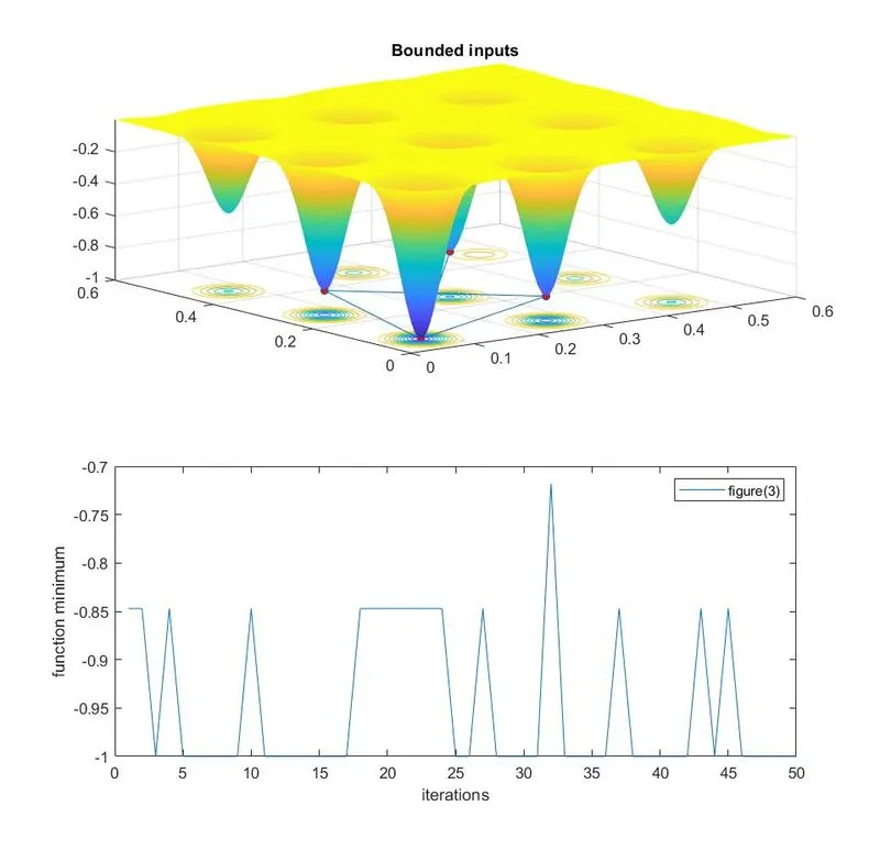
The Study-2 section of the code evaluates the statistical behaviour of stalagmite function with bounded inputs.

• Same procedure as Study_1 section but as lower and upper bounds are taken into consideration,there is a change in the ga syntax :

tic
for i=1:num_cases
[inputs_b,fopt2(i)]=ga(@stalagmite,2,[],[],[],[],[0;0],[1;1]);
xopt2(i)=inputs_b(1);
yopt2(i)=inputs_b(2);
end
study2_time=toc
figure(3)
subplot(2,1,1)
surfc(x,y,f)
hold on 
shading interp
title('Bounded inputs')
plot3(xopt2,yopt2,fopt2,'marker','o','markersize',5,'markerfacecolor','r')
subplot(2,1,2)
plot(fopt2)
xlabel('iterations')
ylabel('function minimum')

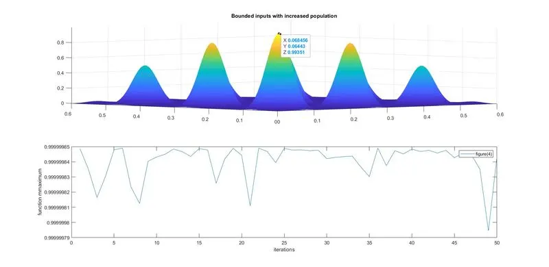
The Study-3 section of the code evaluates the statistical behaviour of stalagmite function with increased population.

• Here,as there is a change in the population size,the ga syntax has been modified;optimoptions ga syntax has been used and global maxima is found:

options =optimoptions('ga');
options =optimoptions(options,'populationsize',300)
tic
for i=1:num_cases
[inputs_c,fopt3(i)]=ga(@stalagmite,2,[],[],[],[],[0;0],[1;1],[],[],options);
xopt3(i)=inputs_c(1);
yopt3(i)=inputs_c(2);
end
study3_time=toc
figure(4)
subplot(2,1,1)
surfc(x,y,-f)
hold on
shading interp
title('Bounded inputs with increased population')
plot3(xopt3,yopt3,-fopt3,'marker','o','markersize',5,'markerfacecolor','r')
subplot(2,1,2)
plot(-fopt3)
xlabel('iterations')
ylabel('function mmaximum')
legend('figure(4)','Location','northeast')

Output:

Results:

From the above output,it is clear that the results are less accurate in case of unbounded inputs as compared to the evaluation of the statistical behaviour of stalagmite function with bounded inputs.

However,with the increase in population with bounded inputs ,we get far better results with the global maxima defined at only one specific point.

• References

Find minimum of function using genetic algorithm - MATLAB ga - MathWorks Deutschland

Genetic Algorithms - Introduction (tutorialspoint.com)