Week 3 - Solving second order ODEs

Aim: To write a MATLAB program that will simulate the motion of a pendulum .

Objectives:

• Write a program that solves the ODE representing the equation of motion of a simple pendulum with damping effect.
• Simulate the motion between 0 to 20 seconds for an angular displacement=0,angular velocity=3 rad/s at time t=0.

Governing equation:

The equation of motion of a simple pendulum (with damping effect) is shown below:

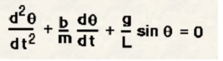
Where:

b stands for the damping coefficient.

m is the mass of the ball hanging at the end the pendulum( in kg).

L is the length of the pendulum(in m)

g is the acceleration due to gravity(in m/s^2)

`theta` is the angular displacement

Theory:

A simple pendulum consists of a ball (of mass m) hanging from a massless string (of length L) , fixed at a pivot point as shown in the figure below.

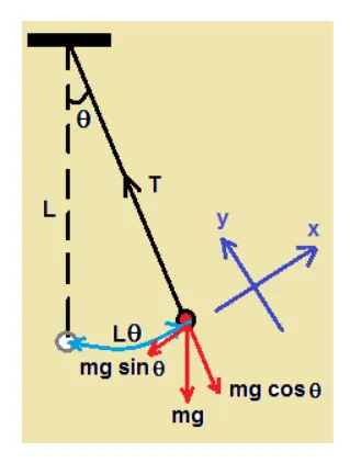
When the pendulum is displaced to an initial displacement and released,it will swing back and forth with a periodic motion.

By simply applying Newton's second law for rotational systems,the equation of motion for the pendulum may be obtained:

`-mg sin(theta)L=mgL^2 (d^2theta //dt^2)` and rearranged as `d^2theta//dt^2+g/l*sin(theta)=0``.

And with small angular displacement,we get: `d^2theta//dt^2+g/l*(theta)=0`

If the damping effect is taken into account,we get our governing equation:

Procedure:

In this project ,a function named ode_func has been written to solve the equation of motion of simple pendulum with damping effect.

That function will be called later in the main program using the matlab inbuilt solver Ode45.

Once this ODE solved,we get ,for each simulation second, a couple of angular displacement and angular velocity.

These values will be used in plotting both ' the angular displacement vs time ' and 'angular velocity vs time 'graphs

And finally,an animation will be made to show the simulation of the motion of the pendulum.

Coding section:

As said previously, a matlab function has been written to be called later in the main program for solving the ODE.

Function code:

function dtheta_dt=ode_func(t,theta,b,g,l,m)
theta1=theta(1);
theta2=theta(2);
dtheta1_dt=theta2;
dtheta2_dt=(-b/m)*theta2-(g/l)*sin(theta1);
dtheta_dt=[dtheta1_dt;dtheta2_dt];
end

Main code:

clear all
close all
clc

%Declaration of input parameters
b=0.05;   %damping coeff.
g=9.81;  %gravitational acceleration in m/s^2
l=1;     %length of the pendulum in m
m=0.1;    % mass in kg
%Initial conditions
theta_0=[0;3];
%time points
tspan=linspace(0,20,200);
%Solve Ode
[t,results]=ode45(@(t,theta)ode_func(t,theta,b,g,l,m),tspan,theta_0)
figure(1)
%Plotting Angular displacement vs time
plot(t,results(:,1),'color','b')
hold on
%Plotting angular velocity vs time
plot(t,results(:,2),'color','r')
ylabel('Angular Displacement & Angular Velocity')
xlabel('Time points')
ct=1;
for i=1:length(tspan)
    %Declaration of the coordinates of the two end points of the pendulum
    x0=0;
    y0=0;
    x=-l*sin(results(i,1));
    y=-l*cos(results(i,1));
    figure(2)
    %Plotting the support rod
    plot([-1,1],[0,0],'color','b','linewidth',6)
       hold on
       %plot the pendulum rod
     plot([x0,x],[y0,y],'color','b','linewidth',2)
     %Plot the ball withw a marker symbol
    plot(x,y,'o','MarkerSize',20,'MarkerFaceColor','r')
   pause(0.005)
   %set the axis
    axis([-2 2 -2 2])
    hold off
M(ct)=getframe(gcf)
ct=ct+1;
end
movie(M)
videofile=VideoWriter('pendulum_ode45.avi','Uncompressed AVI');
open(videofile)
writeVideo(videofile,M)
close(videofile)

Step-wise explanation of the code:

• First of all, for starting a code in MATLAB, it’s highly recommended to use these three basics commands namely:"clc" to clear the command window, “clear all "to completely clear the workspace and ,''close all" to close all the graphs.
• Then input parameters( mass of the ball,length of the pendulum,damping coeficient and gravitational acceleration ) are declared.
• And then the initial conditions(initial angular displacement and initial angular velocity) and the time points(linspace array from 1 to 20 s containing 200 values) are decleared as per the objectives of the project.
• Now the function named ode_func is called to solve the ODE with the help of the Matlab inbuit solver Ode45.
• Once the ODE solved, plotting of "the angular displacement vs time" and "angular velocity vs time" graphs is done.
• A "for loop" is written to show the location of the pendulum at each instant of the oscillation.
• Axes are set.
• A Matlab movie is created to show the simulation in an animation.

Output:

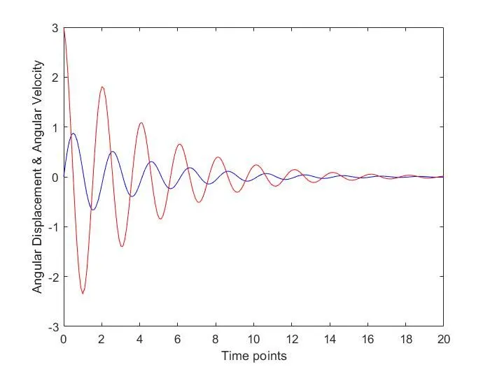
The above graph shows the change of angular displacement with respect to time in blue and the change of the angular velocity with respect to time in red.

Results:

The output shows that both the angular velocity and angular displacement decrease with time as aresult of damping effect.

The results of the simulation of the motion of the pendulum between 0-20 sec, for angular displacement=0,angular velocity=3 rad/sec at time t=0 can be wiewed by simply clicking the following link:https://drive.google.com/file/d/1pATGTqUF6LQvMyrv23gLAJWfm0b_HUWi/view?usp=sharing