Week 3 - Solving second order ODEs
Aim: To write a program in Python that will simulate the motion of a pendulum.
Objectives:
- Write a program that solves the ODE representing the equation of motion of a simple pendulum with damping effect.
- Simulate the motion between 0 to 20 seconds for an angular displacement=0, angular velocity=3 rad/s at time t=0.
Governing equation:
The equation of motion of a simple pendulum with damping effect) is shown below:
`(d^2 (theta))/dt^2+b/m*(d(theta))/dt+g/l*sin(theta)=0`
Where:
b stands for the damping coefficient.
m is the mass of the ball hanging at the end the pendulum (in kg).
L is the length of the pendulum (in m)
g is the acceleration due to gravity (in m/s^2)
`theta` is the angular displacement
Theory:
A simple pendulum consists of a ball (of mass m) hanging from a massless string (of length L), fixed at a pivot point as shown in the figure below.
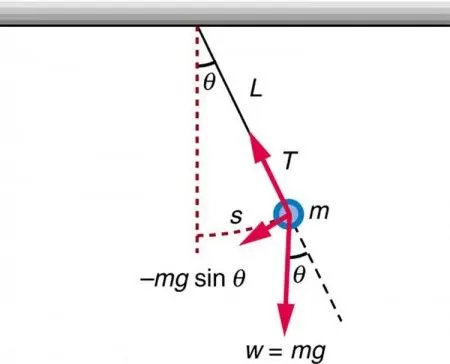
When the pendulum is displaced to an initial displacement and released, it will swing back and forth with a periodic motion.
By simply applying Newton's second law for rotational systems, the equation of motion for the pendulum may be obtained:
`-mg*sin(theta)*L=m*l^2*(d^2(theta)) /dt^2` and rearranged as:`(d^2(theta))/dt^2+g/l*sin(theta)=0`
And with small angular displacement, we get: `(d^2(theta))/dt^2+g/l.theta=0`
If the damping effect is taken into account, we get our governing equation:
`(d^2 (theta))/dt^2+b/m*(d(theta))/dt+g/l*sin(theta)=0`
Procedure:
In this project, a function named "Model" has been written to solve the equation of motion of simple pendulum with damping effect.
Once this ODE solved, we get ,for each time value, a couple of angular displacement and angular velocity.
These values will be used in plotting both ‘the angular displacement vs time ' and 'angular velocity vs time 'graphs
And finally, an animation will be made to show the simulation of the motion of the pendulum.
Coding section:
A Python function has been written to be called later in the main program for solving the ODE.
def Model(theta,t,b,g,l,m):
 	theta1=theta[0]
 	theta2=theta[1]
 	dtheta1_dt=theta2
 	dtheta2_dt=-(b/m)*theta2-(g/l)*math.sin(theta1)
 	dtheta_dt=[dtheta1_dt,dtheta2_dt]
 	return dtheta_dt
Main code:
import math
import matplotlib.pyplot as plt
import numpy as np
from scipy.integrate import odeint
def Model(theta,t,b,g,l,m):
 	theta1=theta[0]
 	theta2=theta[1]
 	dtheta1_dt=theta2
 	dtheta2_dt=-(b/m)*theta2-(g/l)*math.sin(theta1)
 	dtheta_dt=[dtheta1_dt,dtheta2_dt]
 	return dtheta_dt


 	# Damping coefficient
b=0.05
#Acelearation due gto gravity(m/s^2)
g=9.81
#length of the pendulum(m)
l=1
#Mass of
m=1
#Initial condition
theta_0=[0,3]
#Time points
t=np.linspace(0,20,40)
#Solve ODE
theta=odeint(Model,theta_0,t,args=(b,g,l,m))
plt.figure()
#Plotting Angular displacement vs time
plt.plot(t,theta[:,0],'b-',label=r'$\frac{d\theta_1}{dt}=\theta2$')
#plotting angular velocity vs time
plt.plot(t,theta[:,1],'r--',label=r'$\frac{d\theta_2}{dt}=-\frac{b}{m}\theta_2-\frac{g}{L}sin\theta_1$')
#Labelling x-axis
plt.xlabel('time')
#Labelling x-axis
plt.ylabel('Angular Displacement and Angular velocity')
#Labelling x-axis

plt.legend(loc='best')
plt.show()
#Cordinates of the fixed end point of the pendulum
x0=0
y0=0
ct=1
for i in theta[:,0]:
	#Definition of the coordinates moving end point of the pendulum

	x=l*math.sin(i)
	y=-l*math.cos(i)

	#Creating figure window for at each iteration
	plt.figure()
	#plotting the fixed support
	plt.plot([-0.3,0.3],[0,0],'k-',linewidth=10)
	#plotting the string or rod
	plt.plot([x0,x],[y0,y],'r-',linewidth=6)
	filename=str(ct)+'.png'
	#Saving plots with their corresponding filename
	#Plotting the ball
	plt.plot(x,y,'o','b.',markersize=20)
	#Titling the plots
	plt.title('Simple pendulum simulation')
	#Setting x-axis limits
	plt.xlim([-1.5,1.5])
		#Setting y-axis limits

	plt.ylim([-2,2])
	plt.savefig(filename)

	ct=ct+1

#Displaying the plots
plt.show()
Step-wise explanation of the code:
- First of all, "math "module is imported as mathematical tasks with trigonometric functions have been performed in the program.
- Secondly "matplotlib" and "numpy" modules have been also imported to respectively perform plotting tasks and to perform operations on arrays.
- "odeint" library " from "scipy" has also been imported to solve the differential equation.
- Then input parameters( mass of the ball,length of the pendulum,damping coeficient and gravitational acceleration ) are declared.
- And then the initial conditions(initial angular displacement and initial angular velocity) and the time points(linspace array from 1 to 20 s containing 40 values) are decleared as per the objectives of the project.
- Now the function named Model is written and called to solve the ODE with the help of the odeint function from scipy module.
- Once the ODE solved, plotting of "the angular displacement vs time" and "angular velocity vs time" graphs is done.
- A "for loop" is written to show the location of the pendulum at each instant of the oscillation;images at each iteration are saved and an animationgif is generated out of them.
- Axes limits are set.
Output:
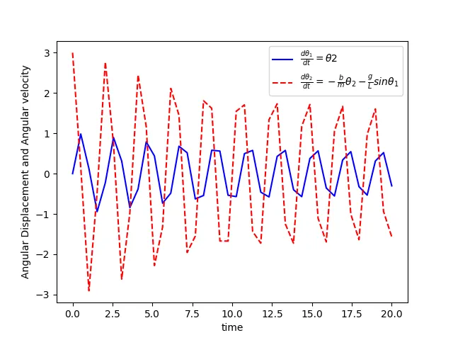
The above graph shows the change of angular displacement with respect to time in blue and the change of the angular velocity with respect to time in red.
Results:
The output shows that both the angular velocity and angular displacement decrease with time as a result of damping effect.
The results of the simulation of the motion of the pendulum between 0-20 sec, for angular displacement=0, angular velocity=3 rad/sec at time t=0 can be viewed by simply clicking on the following link:https://drive.google.com/file/d/17dtChMCWtkL_McQIt8PkD89PHvmi8Kzl/view?usp=sharing