Week 5 - Curve fitting
Aim: To write a code in Python to fit a linear and nth order polynomial for Cp data.
Objectives:
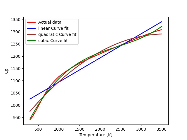
- Write a python code to fit a linear and cubic polynomial for the Cp data. Explain if your results are good or bad.
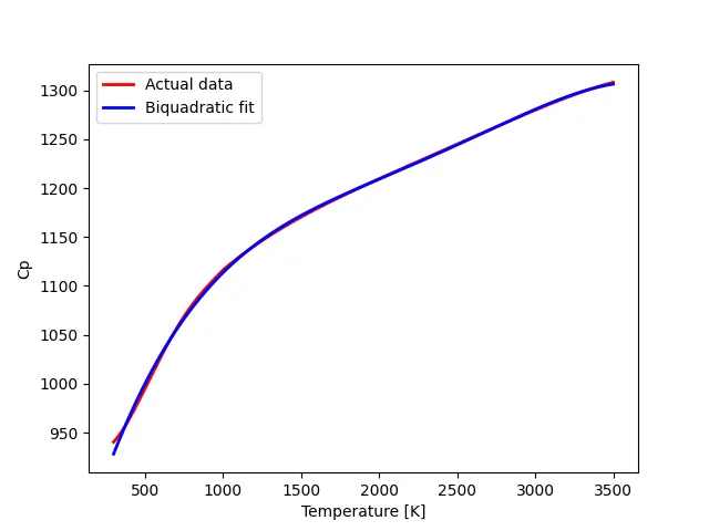
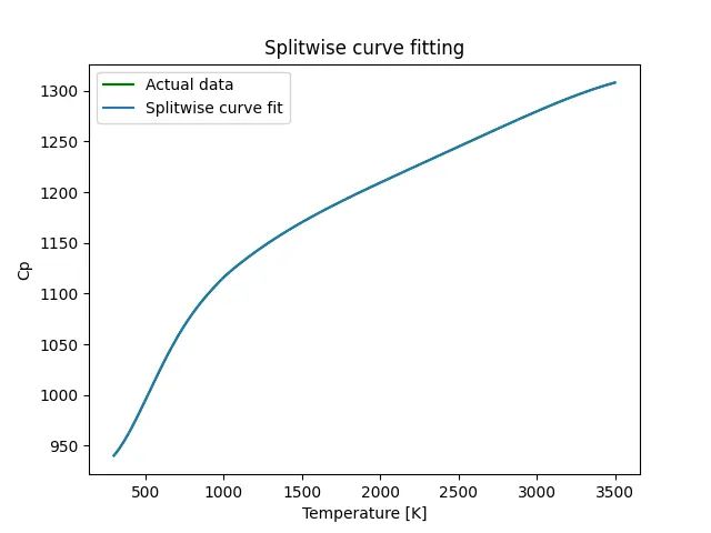
- Show empirically how well your curve has been fit.
Theory:
Curve fitting can be defined as the process of finding an approximate mathematical model that expresses the relationship between a dependant variable y and a single independent variable x and estimating the values of its parameters using non-linear regression.
In other words, it is the process of constructing a curve that has the best fit with a series of data points.
It’s basically a statistical model which establishes a discrepancy between the observed values and those that would be expected of the model in a normal distribution case.
Answers to asked questions:

- popt is a 1*n array that contains the optimal values for the parameters so that the sum of the squared residuals of f(xdata,*popt)-ydata is minimized.
- pcov is an array that represents the estimated covariance of popt. The diagonals provide the variance of the parameter estimate.
- The asterisk in "*popt" notation will expand a list of values into the arguments of the function.
- np.array(temperature) stores the temperature values in form of array and passes it to the function numpy.
Coding section:
The program below displays in a first time the linear,cubic,quadratic and biquadratic curve fits of cp data and at the end,the curve fit using the splitwise method.
Code:
"""
Curve fitting challenge
"""

import numpy as np
import matplotlib.pyplot as plt
from scipy.optimize import curve_fit
#Curve fit linear function
def func_1(t,a,b):
	return a*t+b
#Curve fit quadratic function
def func_2(t,a,b,c):
	return a*pow(t,2)+b*t+c

#Curve fit cubic function
def func_3(t,a,b,c,d):
	return a*pow(t,3)+b*pow(t,2)+c*t+d

#Curve fit with biquadratic function
def func_4(t,a,b,c,d,e):
	return a*pow(t,4)+b*pow(t,3)+c*pow(t,2)+d*t+e
#Reading thermodynamic  data file


def read_file():
	temperature=[]
	cp=[]
	for line in open ('data','r'):
		values=line.split(',')
		temperature.append(float(values[0]))
		cp.append(float(values[1]))
	return [temperature,cp]


#Reading thermodynamic  data file

def read_file():
	temperature=[]
	cp=[]
	for line in open ('data','r'):
		values=line.split(',')
		temperature.append(float(values[0]))
		cp.append(float(values[1]))
	return [temperature,cp]


#Main program

temperature,cp=read_file()
popt1,pcov1=curve_fit(func_1,temperature,cp)
fit_cp_1=func_1(np.array(temperature),*popt1)


popt2,pcov2=curve_fit(func_2,temperature,cp)
fit_cp_2=func_2(np.array(temperature),*popt2)

popt3,pcov3=curve_fit(func_3,temperature,cp)
fit_cp_3=func_3(np.array(temperature),*popt3)

popt4,pcov4=curve_fit(func_4,temperature,cp)
fit_cp_4=func_4(np.array(temperature),*popt4)


plt.plot(temperature,cp,color="red",linewidth=2)
plt.plot(temperature,fit_cp_1,color="blue",linewidth=2)
plt.plot(temperature,fit_cp_2,color="brown",linewidth=2)
plt.plot(temperature,fit_cp_3,color="green",linewidth=2)

plt.legend(['Actual data','linear Curve fit','quadratic Curve fit','cubic Curve fit'])
plt.xlabel('Temperature [K]')
plt.ylabel('Cp')
plt.show()


#Biquadratic curve fit
plt.figure()
plt.plot(temperature,cp,color="red",linewidth=2)
plt.plot(temperature,fit_cp_4,color='blue',linewidth=2)
plt.legend(['Actual data','Biquadratic fit'])
plt.xlabel('Temperature [K]')
plt.ylabel('Cp')
plt.show()


"""
Splitwise Method
"""
plt.figure()

a=0
b=399
fit_cp=[]

for i in range(0,8):

     c=temperature[a:b+1]
     d=cp[a:b+1]

     popt,pcov=curve_fit(func_3,c,d)
     z=func_3(np.array(c),*popt)

     for j in z:
     	fit_cp.append(j)

     a=b+1
     b=b+400
plt.figure()
plt.plot(temperature,cp,color='green',linewidth=1.5)
plt.plot(temperature,fit_cp)
plt.legend(['Actual data','Splitwise curve fit'])
plt.xlabel('Temperature [K]')
plt.ylabel('Cp')
plt.title('Splitwise curve fitting')
plt.show()
Explanation of the code:
- First of all,necessary modules have been imported:
- Firstly, "matplotlib" and "numpy" modules have been imported to respectively perform plotting tasks and to perform operations on arrays.
- Secondly,"curve_fit" module " from "scipy.optimize" has also been imported perform curve fitting operations.
import numpy as np
import matplotlib.pyplot as plt
from scipy.optimize import curve_fit- Then the linear,quadratic,cubic and biquadratic curve fit functions have been defined as func_1,func_2,func_3 and func_4 respectively.
def func_1(t,a,b):
	return a*t+b
#Curve fit quadratic function
def func_2(t,a,b,c):
	return a*pow(t,2)+b*t+c

#Curve fit cubic function
def func_3(t,a,b,c,d):
	return a*pow(t,3)+b*pow(t,2)+c*t+d

#Curve fit with biquadratic function
def func_4(t,a,b,c,d,e):
	return a*pow(t,4)+b*pow(t,3)+c*pow(t,2)+d*t+e
#Reading thermodynamic  data file
- A function named read_file() has been defined to open and read the cp data file and to append the values of temperature and cp to the variables of the same name previously defined as empty arrays.
def read_file():
	temperature=[]
	cp=[]
	for line in open ('data','r'):
		values=line.split(',')
		temperature.append(float(values[0]))
		cp.append(float(values[1]))
	return [temperature,cp]
- In the main program,for each curve fitting defined function,the curve_fit function is used to return two values :The popt and pcov whose meaning has been given in the begining of this report.
- Similary the fit cp value is computed at each level using a particular syntax.
temperature,cp=read_file()
popt1,pcov1=curve_fit(func_1,temperature,cp)
fit_cp_1=func_1(np.array(temperature),*popt1)


popt2,pcov2=curve_fit(func_2,temperature,cp)
fit_cp_2=func_2(np.array(temperature),*popt2)

popt3,pcov3=curve_fit(func_3,temperature,cp)
fit_cp_3=func_3(np.array(temperature),*popt3)

popt4,pcov4=curve_fit(func_4,temperature,cp)
fit_cp_4=func_4(np.array(temperature),*popt4)
- Once the different temperature values and their corresponding cp values are known,temperature vs cp curves are plotted for the actual data set,the linear,quadratic,cubic and biquadratic fitting defined functions.
plt.plot(temperature,cp,color="red",linewidth=2)
plt.plot(temperature,fit_cp_1,color="blue",linewidth=2)
plt.plot(temperature,fit_cp_2,color="brown",linewidth=2)
plt.plot(temperature,fit_cp_3,color="green",linewidth=2)

plt.legend(['Actual data','linear Curve fit','quadratic Curve fit','cubic Curve fit'])
plt.xlabel('Temperature [K]')
plt.ylabel('Cp')
plt.show()


#Biquadratic curve fit
plt.figure()
plt.plot(temperature,cp,color="red",linewidth=2)
plt.plot(temperature,fit_cp_4,color='blue',linewidth=2)
plt.legend(['Actual data','Biquadratic fit'])
plt.xlabel('Temperature [K]')
plt.ylabel('Cp')
plt.show()- A number of line codes has also been written to illustrate the splitwise method which consists of dividing the complete data into a number of parts followed by local curve fitting on each part using a given fitting function:Here I used the cubic curve fitting function
plt.figure()

a=0
b=399
fit_cp=[]

for i in range(0,8):

     c=temperature[a:b+1]
     d=cp[a:b+1]

     popt,pcov=curve_fit(func_3,c,d)
     z=func_3(np.array(c),*popt)

     for j in z:
     	fit_cp.append(j)

     a=b+1
     b=b+400
plt.figure()
plt.plot(temperature,cp,color='green',linewidth=1.5)
plt.plot(temperature,fit_cp)
plt.legend(['Actual data','Splitwise curve fit'])
plt.xlabel('Temperature [K]')
plt.ylabel('Cp')
plt.title('Splitwise curve fitting')
plt.show()
Output:
Conclusion:
From the different screenshots of the ouput,we can clearly conclude that the goodness of the fit increases with the increase of the order of the fitting polynomial:The biquadratic curve fit is better than to the cubic curve fit which is better as compared to the linear one.
To find the best fit,one can use the splitwise method which consists of dividing the complete data into a number of parts followed by local curve fitting on each part.