Week 2 Air standard Cycle

OTTO CYCLE P V DIAGRAM

AIM

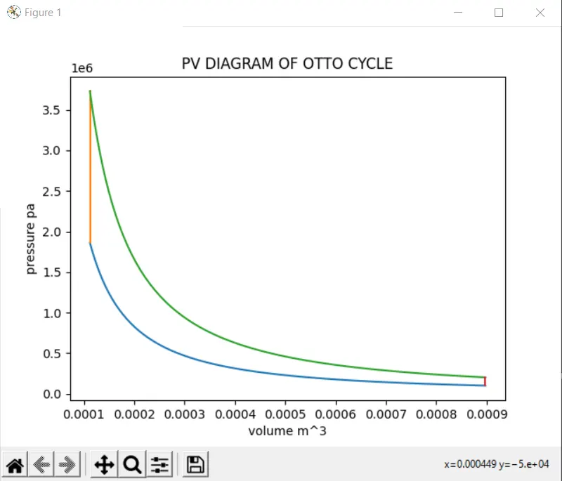
To plot the pressure- volume graph and to find thermal efficency of Otto cycle using python

OBJECTIVE

DESCRIPTION

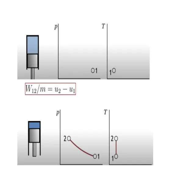
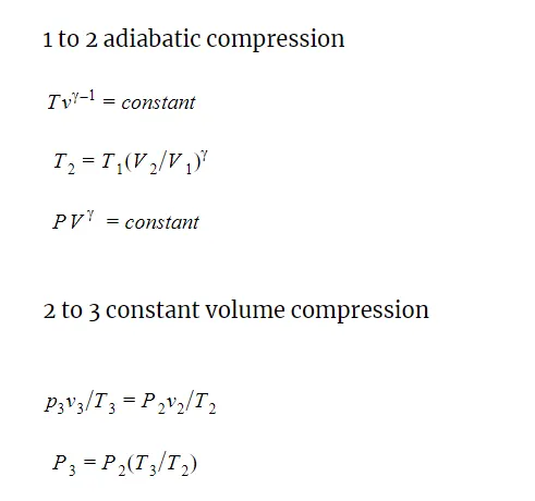
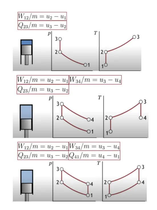
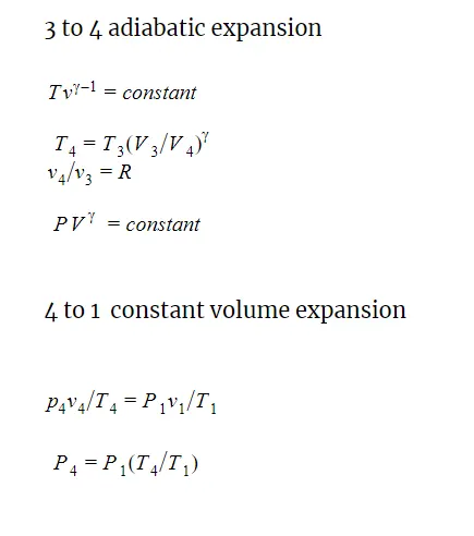
The Otto cycle is consists of

Process 1–2 is an adiabatic (isentropic) compression of the charge as the piston moves from bottom dead center (BDC) to top dead center (TDC).

Crank angle 180 to 0

V1p1 to v2p2

Process 2–3 is a constant-volume heat transfer to the working gas from an external source while the piston is at top dead center. This process is intended to represent the ignition of the fuel-air mixture and the subsequent rapid burning.

V2p2 to v3p3

Process 3–4 is an adiabatic (isentropic) expansion (power stroke).

Crank angle 0 to 180

V3p3 tov4p4

Process 4–1 completes the cycle by a constant-volume process in which heat is rejected from the air while the piston is at the bottom dead center.

V4p4 to v1p1

EQUATIONS

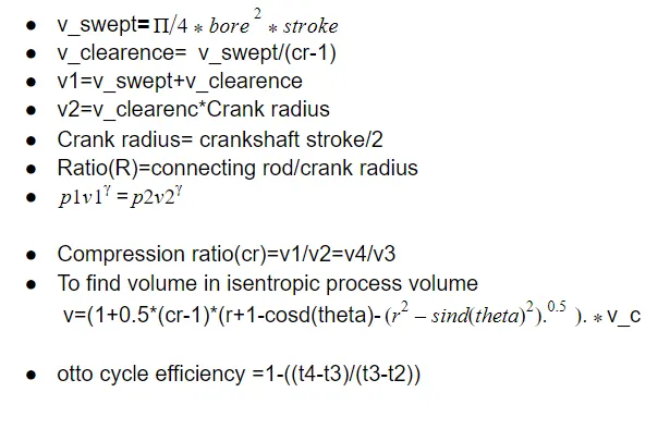
• Bore-bore is the diameter of each cylinder
• stroke-stroke is the distance within the cylinder the piston travels
• Swept volume-volume through which a piston or plunger moves as it makes a stroke.
• Clearance volume- volume between the cylinder head and the piston when the piston is at tdc.
• Compression ratio-The ratio of clearance volume to the swept volume determines the compression ratio of the engine.

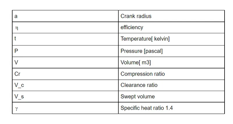
ALGORITHAM

Program algorithm

Step 1;start the program

Step2;import math. command is used to call trigonometric functions(mathematical functions.calculations and import matplotlib.pyplot as plt command to plot graphs in programing

Step3;Define a function named engine kinematics using ‘def ’with input of engine parameters like bore,stroke length,rod length and compression ratio.Defining a function will help to achieve a series of values for compression and expansion stroke easily.

step4;Find a [crank radius] and R using equations provided

step5;define clearance and swept volume

Step6;start crank angle[180 degree] and end crank angle[0] values are assigned to variable name sc and ec respectively

Step7;to trace the volume in isentropic processes ,empty array of v is initialized in a range of 0 to a number of values [difference between sc and ec]

Where dtheta=(ec-sc)/(num_values-1)

theta=sc+i*dtheta

term1=0.5*(cr-1)

term2=R+1-math.cos(theta)

term3=pow(R,2)-pow(math.sin(theta),2)

term3=pow(term3,0.5)

v.append((1+term1*(term2-term3))*v_c)

Step9;values appended for each theta by command append ,and returned each value V

Step10; enter given state variables

Step11;enter engine parameters given

Step12;compute state variables at each point using equation thermodynamic fomula

Step13;V compression v expansion find out using defined function

Compression 180 to 0

Expansion 0 to 180

Step14;plot the graph using plt. Command

Step15;x and y labelled

Step16;give title

Step17;plt.show is the command used to plot it and make graph visible

Step19;find thermal efficiency using equation

step20;end the program

PROGRAM

import math
import matplotlib.pyplot as plt
def engine_kinematics(bore,stroke,con_rod,cr,start_crank,end_crank):
      
     a=stroke/2
     R=con_rod/a
    


     v_s=(math.pi*(1/4))*pow(bore,2)*stroke
     v_c=v_s/(cr-1)
     sc=math.radians(start_crank)
     ec=math.radians(end_crank)

     num_values=100
     dtheta=(ec-sc)/(num_values-1)
     v=[]
     for i in range(0,num_values):
          
          theta=sc+i*dtheta
          term1=0.5*(cr-1)
          term2=R+1-math.cos(theta)
          term3=pow(R,2)-pow(math.sin(theta),2)
          term3=pow(term3,0.5)
          v.append((1+term1*(term2-term3))*v_c)

     return (v)        


#inputs        
t1=500
gamma=1.4
t3=2300
p1=101325

#geometric parameters
bore=0.1
stroke=0.1
con_rod=0.15
cr=8

#volume computation



v_s=math.pi*(1/4)*pow(bore,2)*stroke
v_c=v_s/(cr-1)
v1=v_c+v_s
#state point 2
v2=v_c
#p2v2^gamma=p1v1^gamma
p2=p1*pow(v1,gamma)/pow(v2,gamma)

#p2v2/t2=p1v2/t1
rhs=p1*v1/t1
t2=p2*v2/rhs
v_compression=engine_kinematics(bore,stroke,con_rod,cr,180,0)
constant=p1*pow(v1,gamma)
p_compression=[]

for V in v_compression:
     p_compression.append(constant/pow(V,gamma))
#state point3
v3=v2
#p3v3/t3=p2v2/t2
rhs=p2*v2/t2
p3=rhs*t3/v3
v_expansion=engine_kinematics(bore,stroke,con_rod,cr,0,180)

#(p3>p2)
constant=p3*pow(v3,gamma)
p_expansion=[]
for V in v_expansion:
     p_expansion.append(constant/pow(V,gamma))
#sate point4
v4=v1
#p4v4^gamma=p3v3^gamma
p4=p3*pow(v3,gamma)/pow(v4,gamma)
#p4v4/t4=rhs
t4=p4*v4/rhs
#thermal efficency
eth=1-((t4-t1)/(t3-t2))
print(eth)

plt.plot(v_compression,p_compression)
plt.plot([v2,v3],[p2,p3])
plt.plot(v_expansion,p_expansion)
plt.plot([v4,v1],[p4,p1])
plt.xlabel('volume m^3')
plt.ylabel('pressure pa')
plt.title('PV DIAGRAM OF OTTO CYCLE')
plt.show()
     
   

OUTPUT

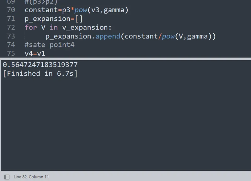
Thermal Efficency

CONCLUSION

Pv graph of otto cycle plotted

Thermal efficiency calculated

The Python program has been executed successfully and output verified