Week 2 Air standard Cycle

                                               Otto cycle

Aim: -

Writing a Python program that can solve an otto cycle and make plots for it.

Objectives: -

1. Able to find start & end-state properties for different processes in the otto cycle.
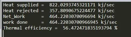
2. Able to find net-work done by the system, the thermal efficiency of the engine.
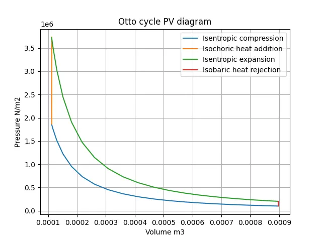
3. Able to plot the Pressure vs Volume (P/V) diagram.

Description: -

            Otto cycle is also called a constant volume air standard cycle on which petrol & gas engines will work.

Procedure: -

1. Define input variables & geometry.
2. use engine kinematics formulae to find the path of the process undergone while compression and expansion.
3. Find the unknown variables using thermodynamic relations.
4. Extract the results.
5. Plot results on Pressure vs Volume (P/V) graph. 

Main program: -

# otto cycle simulator

import math                         # importing math library
import matplotlib.pyplot as plt     # importing ploting library  

def engine_kinmatics(bore, stroke, con_rod_l, cr, start_crank, end_crank):
	# engine kinematics
	# Geometric parameters
	a = stroke/2
	R = con_rod_l/a
	#volume parameters
	v_s = (math.pi/4)*(bore**2)*stroke        # swept volume
	v_c = v_s/(cr-1)                          # clearance volume
	# Crank angles
	sc  = math.radians(start_crank)           # starting crank angle
	ec  = math.radians(end_crank)             # ending crank angle
	num_values = 25
	dtheta = (ec-sc)/(num_values-1)
	V = []

	for i in range(0,num_values):
		theta = sc + i*dtheta
		term1 = 0.5*(cr-1)
		term2 = R + 1 - math.cos(theta)
		term3 = pow((R**2)-(math.sin(theta)**2),0.5)

		V.append((1 + term1*(term2 - term3))*v_c) 
	return(V)


# inputs
p1 = 101325     # inlet pressure
t1 = 500        # inlet temperature
gamma = 1.4     
t3 = 2300       # maximum temperature ignition temperature

# geometric parameters

bore = 0.1
stroke = 0.1
con_rod_l = 0.15    # connecting rod length
cr = 8              # compression ratio

# volume computation
v_s = (math.pi/4)*(bore**2)*stroke
v_c = v_s/(cr-1)

# state point 1 calculation
v1  = v_c + v_s

# state point 2 after compression
v2 = v_c
# p2v2^gamma  =  p1v1^gamma
p2 = p1*(v1**gamma)/(v2**gamma)
# p2v2/t2 = p1v1/t1  || rhs = p1v1/t1  || p2v2/t2 = rhs || t2 = p2v2/rhs
rhs = p1*v1/t1
t2 = p2*v2/rhs

V_compression = engine_kinmatics(bore, stroke, con_rod_l, cr, 180, 0)
constant = p1*(v1**gamma)
P_compression = []

for v in V_compression:
	P_compression.append(constant/(v**gamma))

# state poit 3 after heat addition
v3 = v2
# p3v3/t3 = p2v2/t2  || rhs = p2v2/t2  || p3 =  rhs*t3/v3
rhs = p2*v2/t2
p3  = rhs*t3/v3

V_expansion = engine_kinmatics(bore, stroke, con_rod_l, cr, 0, 180)
constant = p3*(v3**gamma)
P_expansion = []

for v in V_expansion:
	P_expansion.append(constant/(v**gamma))

# state point 4 after expansion
v4 = v1
# p4v4^gamma  = p3v3^gamma
p4 = p3*(v3**gamma)/(v4**gamma)
# p4v4/t4 = rhs
t4 = p4*v4/rhs

#work done, efficency
m = 1;             # mass flow rate kg/sec
cv = 714;          # specific heat at constant volume j/kg K
Heat_supplied =  m*cv*(t3-t2)/1000        # heat supplied to system kj/sec
Heat_rejected = m*cv*(t4-t1)/1000         # heat rejected by system kj/sec
Net_Work = Heat_supplied-Heat_rejected    # net work done by system
W = m*cv*((t3-t2)-(t4-t1))/1000          # work done kj/sec
Thermal_efficiency = (1-(1/(cr**(gamma-1)))) * 100    # Thermal efficency
print('Heat supplied = ',Heat_supplied,'kj/sec')
print('Heat rejected = ',Heat_rejected,'kj/sec')
print('Net_Work      = ',Net_Work,'kj/sec')
print('work done     = ',W,'kj/sec')
print('Thermal efficiency = ',Thermal_efficiency,'%')

# ploting results
plt.figure()
plt.plot(V_compression,P_compression,label='Isentropic compression')
plt.plot([v2,v3],[p2,p3],label='Isochoric heat addition')
plt.plot(V_expansion,P_expansion,label='Isentropic expansion')
plt.plot([v4,v1],[p4,p1],label='Isobaric heat rejection')
plt.xlabel('Volume m3')    
plt.ylabel('Pressure N/m2') 
plt.title('Otto cycle PV diagram')  
plt.legend() 
plt.grid('on')
plt.show()

Output/Results: -

Graphs: -

Conclusions: -

1. The actual Pressure vs Volume (P/V) diagram is plotted.