Week 12 - Validation studies of Symmetry BC vs Wedge BC in OpenFOAM vs Analytical H.P equation
AIM: To simulate the axis-symmetric flow by applying the Symmetry Boundary Condition. Also to simulate for the below-mentioned angles using both symmetry and wedge boundary conditions.
OBJECTIVE:
1. Do the simulation for the below mentioned angles using both symmetry and wedge boundary conditions
Angles to test:
- Ten degrees
- twenty five degress
- fourty five degrees
2. Validate Hydro-dynamic length with the numerical result.
THEORY AND EXPLANATION:
Axi-symmetric flow: A flow pattern is axisymmetric when it is identical in every plane that passes through a certain straightline. The straight-line in question is referred to as the symmetry axis. Every longitudinal plane through the axis would exhibit the same streamline pattern.
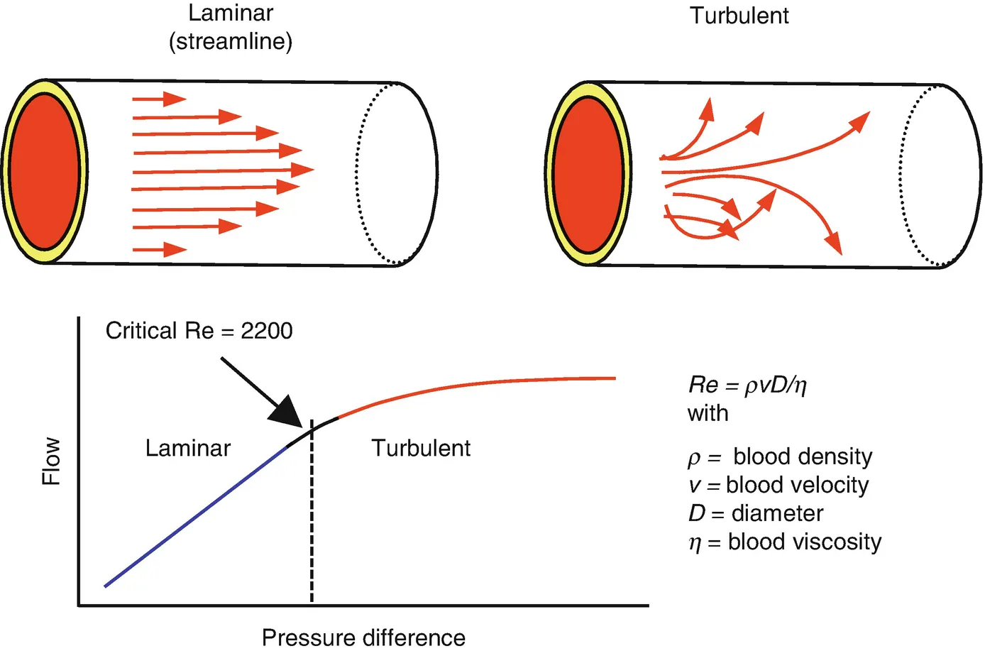
Laminar Flow: In fluid dynamics, laminar flow is characterized by fluid particles following smooth paths in layers, with each layer moving smoothly past the adjacent layers with little or no mixing. At low velocities, the fluid tends to flow without lateral mixing, and adjacent layers slide past one another like playing cards. There are no cross-currents perpendicular to the direction of flow, nor eddies or swirls of fluids. In laminar flow, the fluid particles' motion is very orderly, with particles close to a solid surface moving in straight lines parallel to that surface.
Laminar flow is a flow regime characterized by high momentum diffusion and low momentum convection. When a fluid flows through a closed channel such as a pipe or between two flat plates, either of two types of flow may occur depending on the fluid's velocity and viscosity: laminar flow or turbulent flow. Laminar flow occurs at lower velocities, below a threshold at which the flow becomes turbulent. The velocity is determined by a dimensionless parameter characterizing the flow called the Reynolds number, which also depends on the viscosity and density of the fluid and dimensions of the channel.
Reynolds Number: The Reynolds number (Re) helps predict flow patterns in different fluid flow situations At low Reynolds numbers, flows tend to be dominated by laminar (sheet-like) flow, while at high Reynolds numbers, flows tend to be turbulent. The turbulence results from differences in the fluid's speed and direction, which may sometimes intersect or even move counter to the flow's overall direction (eddy currents). These eddy currents begin to churn the flow, using up energy in the process, which for liquids increases the chances of cavitation. Reynolds numbers are an important dimensionless quantity in fluid mechanics.
Comparison between Laminar flow and Turbulent flow:
Given below are equations for pressure drop for an incompressible laminar flow through a pipe:
△ P = P1 − P2 = 8μLVavg / R^2 = 32μLVavg / D^2
Where,
μ = dynamic viscosity
L= length of the pipe
Vavg= average velocity
D= Diameter of the pipe
Laminar Flow Through pipe:
Consider the steady, laminar, incompressible flow of fluid with constant properties in the fully developed region of a straight circular pipe. The momentum equation obtained by applying a momentum balance to a differential volume element, and also the velocity profile is obtained by solving it. Then it is used to obtain a relation for the friction factor. An important aspect of the analysis here is that it is one of the few available for viscous flow.
In fully developed laminar flow, each fluid particle moves at a constant axial velocity along a streamline and the velocity profile u(r) remains unchanged in the flow direction. There is no motion in the radial direction, and thus the velocity component in the direction normal to the pipe axis is everywhere zero. There is no acceleration since the flow is steady and fully developed.
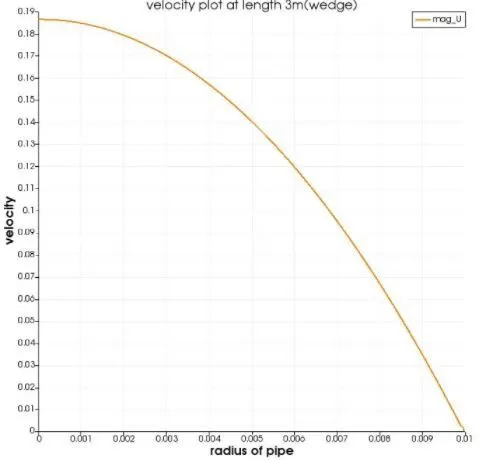
The velocity profile is fully developed laminar flow in a pipe is parabolic with a maximum at the centerline and a minimum (zero) at the pipe wall and is given by the equation as a function of radial distance from the center.
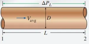
The pressure drop due to viscous effects over the length of the pipe is:
△ P = P1 − P2 = 8μLVavg / R^2
For this simulation of Flow-Through axis-symmetric, all the above formulae are used to simulate the flow. Since the model is axis-symmetric only a small wedge is modeled such that this wedge is a symmetric part of the Cylinder
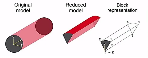
In the above-reduced figure of the axis-symmetric model, the block consists of 6 vertices namely 0,1,2,3,4,5 where the face 012 is Inlet, 345 is the outlet, 1254 is the wall of the cylinder and the 0253 and 0341 is the wedge patch or symmetry patch using icoFoam solver.
The code for symmetry boundary condition(10 degrees):
clear all
close all
clc
%inputs
%diamter of pipe(m)
D = 0.02;
%wedge angle
theta = 10;
%reynolds number
Re = 2100;
%entrance length
Le = 0.06*Re*D;
%length of pipe
L = 3;
%dynamic viscosity of water(NS/m^2)
dynamic_viscosity = 8.9e-4;
%density(kg/m^3)
rho = 997;
%kinematic viscosity(m^2/S)
mu = dynamic_viscosity/rho;
%average_velocity(m/s)
V = Re*mu/D;
%maximum velocity
V_max = 2*V;
%kinematic pressure drop(N/m^2)
delta_p = 32*mu*V*L/D^2;
%radius
R = linspace(0,0.01,20);
for i = 1:length(R)
 %local velocity
 V_local(i) = 2*V*(1-(4*R(i)^2/D^2));

 %wall shear stress
 tau(i) = 16*mu*rho*V*R(i)/D^2;
end
figure(1)
plot(R,V_local)
xlabel('Radius')
ylabel('local velocity')
legend('analytical velocity profile')
figure(2)
plot(R,tau)
xlabel('Radius')
ylabel('wall shear stress')
legend('analytical wall shear stress profile')
%BlockMeshdict file:
%vertices
v_0 = [0 0 0];
v_1 = [0 D/2*cosd(theta/2) D/2*sind(theta/2)];
v_2 = [0 D/2*cosd(theta/2) -D/2*sind(theta/2)];
v_3 = [L 0 0];
v_4 = [L D/2*cosd(theta/2) D/2*sind(theta/2)];
v_5 = [L D/2*cosd(theta/2) -D/2*sind(theta/2)];
%headers
h1 = '/*--------------------------------*- C++ -*----------------------------------*';
h2 = ' ========= |';
h3 = ' \ / F ield |';
h4 = ' \ / O peration |';
h5 = ' \ / A nd |';
h6 = ' \/ M anipulation |';
h7 = '*---------------------------------------------------------------------------*/';
%creating blockmeshdict file
f1 = fopen('blockMeshDict.text','w');
fprintf(f1, '%sn', h1)
fprintf(f1, '%sn', h2)
fprintf(f1, '%sn', h3)
fprintf(f1, '%sn', h4)
fprintf(f1, '%sn', h5)
fprintf(f1, '%sn', h6)
fprintf(f1, '%sn', h7)
fprintf(f1, 'FoamFilen%sn','{')
fprintf(f1, '%10s %13sn', 'version', '2.0;')
fprintf(f1, '%9s %16sn', 'format', 'ascii;')
fprintf(f1, '%8s %22sn', 'class', 'dictionary;')
fprintf(f1, '%9s %24sn', 'object', 'blockMeshDict;')
fprintf(f1, '%sn','}')
h8 = '// * * * * * * * * * * * * * * * * * * * * * * * * * * * * * * * * * * * * * //';
fprintf(f1, '%sn',h8)
fprintf(f1, '%s %5sn', 'convertToMeters', '1;')
fprintf(f1, 'verticesn%sn','(')
fprintf(f1, 't(%d %d %d)n',v_0)
fprintf(f1, 't(%d %d %d)n',v_1)
fprintf(f1, 't(%d %d %d)n',v_2)
fprintf(f1, 't(%d %d %d)n',v_3)
fprintf(f1, 't(%d %d %d)n',v_4)
fprintf(f1, 't(%d %d %d)n',v_5)
fprintf(f1, '%sn',');')
fprintf(f1, 'blocksn%sn','(')
fprintf(f1, 'thex (0 3 5 2 0 3 4 1)(250 50 1)')
fprintf(f1, ' simpleGrading (1 0.2 1)n);n')
fprintf(f1, 'edgesn%sn', '(')
fprintf(f1, 'tarc 1 2 (%d %d %d)n', 0,D/2,0)
fprintf(f1, 'tarc 4 5 (%d %d %d)n);n', L,D/2,0)
fprintf(f1, 'boundaryn')
fprintf(f1,'%sn','(')
fprintf(f1, 'tinletn')
fprintf(f1, 't{n')
fprintf(f1, '%15s %6sn', 'type', 'patch;')
fprintf(f1, '%16sn%12sn', 'faces','(')
fprintf(f1, 'tt(0 1 2 0)n')
fprintf(f1, '%12sn',');')
fprintf(f1, 't}n')
fprintf(f1, 'toutletn')
fprintf(f1, 't{n')
fprintf(f1, '%15s %6sn', 'type', 'patch;')
fprintf(f1, '%16sn%12sn', 'faces','(')
fprintf(f1, 'tt(3 5 4 3)n')
fprintf(f1, '%12sn',');')
fprintf(f1, 't}n')
fprintf(f1, 'ttopn')
fprintf(f1, 't{n')
fprintf(f1, '%15s %6sn', 'type', 'wall;')
fprintf(f1, '%16sn%12sn', 'faces','(')
fprintf(f1, 'tt(4 5 2 1)n')
fprintf(f1, '%12sn',');')
fprintf(f1, 't}n')
fprintf(f1, 'tfrontn')
fprintf(f1, 't{n')
fprintf(f1, '%15s %6sn', 'type', 'symmetry;')
fprintf(f1, '%16sn%12sn', 'faces','(')
fprintf(f1, 'tt(0 3 4 1)n')
fprintf(f1, '%12sn',');')
fprintf(f1, 't}n')
fprintf(f1, 'tbackn')
fprintf(f1, 't{n')
fprintf(f1, '%15s %6sn', 'type', 'symmetry;')
fprintf(f1, '%16sn%12sn', 'faces','(')
fprintf(f1, 'tt(0 2 5 3)n')
fprintf(f1, '%12sn',');')
fprintf(f1, 't}n')
fprintf(f1, 'taxisn')
fprintf(f1, 't{n')
fprintf(f1, '%15s %6sn', 'type', 'empty;')
fprintf(f1, '%16sn%12sn', 'faces','(')
fprintf(f1, 'tt(0 3 3 0)n')
fprintf(f1, '%12sn',');')
fprintf(f1, 't}n')
fprintf(f1, ');n')
fprintf(f1, 'mergePatchPairsn')
fprintf(f1, '(n);n')
h9 = '// ************************************************************************* //';
fprintf(f1,'%s',h9)
fclose(f1)
The code for wedge boundary condition(10 degrees):
clear all
close all
clc
%inputs
%diamter of pipe(m)
D = 0.02;
%wedge angle
theta = 10;
%reynolds number
Re = 2100;
%entrance length
Le = 0.06*Re*D;
%length of pipe
L = 3;
%dynamic viscosity of water(NS/m^2)
dynamic_viscosity = 8.9e-4;
%density(kg/m^3)
rho = 997;
%kinematic viscosity(m^2/S)
mu = dynamic_viscosity/rho;
%average_velocity(m/s)
V = Re*mu/D;
%maximum velocity
V_max = 2*V;
%kinematic pressure drop(N/m^2)
delta_p = 32*mu*V*L/D^2;
%radius
R = linspace(0,0.01,20);
for i = 1:length(R)
 %local velocity
 V_local(i) = 2*V*(1-(4*R(i)^2/D^2));

 %wall shear stress
 tau(i) = 16*mu*rho*V*R(i)/D^2;
end
figure(1)
plot(R,V_local)
xlabel('Radius')
ylabel('local velocity')
legend('analytical velocity profile')
figure(2)
plot(R,tau)
xlabel('Radius')
ylabel('wall shear stress')
legend('analytical wall shear stress profile')
%BlockMeshdict file:
%vertices
v_0 = [0 0 0];
v_1 = [0 D/2*cosd(theta/2) D/2*sind(theta/2)];
v_2 = [0 D/2*cosd(theta/2) -D/2*sind(theta/2)];
v_3 = [L 0 0];
v_4 = [L D/2*cosd(theta/2) D/2*sind(theta/2)];
v_5 = [L D/2*cosd(theta/2) -D/2*sind(theta/2)];
%headers
h1 = '/*--------------------------------*- C++ -*----------------------------------*';
h2 = ' ========= |';
h3 = ' \ / F ield |';
h4 = ' \ / O peration |';
h5 = ' \ / A nd |';
h6 = ' \/ M anipulation |';
h7 = '*---------------------------------------------------------------------------*/';
%creating blockmeshdict file
f1 = fopen('blockMeshDict.text','w');
fprintf(f1, '%sn', h1)
fprintf(f1, '%sn', h2)
fprintf(f1, '%sn', h3)
fprintf(f1, '%sn', h4)
fprintf(f1, '%sn', h5)
fprintf(f1, '%sn', h6)
fprintf(f1, '%sn', h7)
fprintf(f1, 'FoamFilen%sn','{')
fprintf(f1, '%10s %13sn', 'version', '2.0;')
fprintf(f1, '%9s %16sn', 'format', 'ascii;')
fprintf(f1, '%8s %22sn', 'class', 'dictionary;')
fprintf(f1, '%9s %24sn', 'object', 'blockMeshDict;')
fprintf(f1, '%sn','}')
h8 = '// * * * * * * * * * * * * * * * * * * * * * * * * * * * * * * * * * * * * *//';
fprintf(f1, '%sn',h8)
fprintf(f1, '%s %5sn', 'convertToMeters', '1;')
fprintf(f1, 'verticesn%sn','(')
fprintf(f1, 't(%d %d %d)n',v_0)
fprintf(f1, 't(%d %d %d)n',v_1)
fprintf(f1, 't(%d %d %d)n',v_2)
fprintf(f1, 't(%d %d %d)n',v_3)
fprintf(f1, 't(%d %d %d)n',v_4)
fprintf(f1, 't(%d %d %d)n',v_5)
fprintf(f1, '%sn',');')
fprintf(f1, 'blocksn%sn','(')
fprintf(f1, 'thex (0 3 5 2 0 3 4 1)(250 50 1)')
fprintf(f1, ' simpleGrading (1 0.2 1)n);n')
fprintf(f1, 'edgesn%sn', '(')
fprintf(f1, 'tarc 1 2 (%d %d %d)n', 0,D/2,0)
fprintf(f1, 'tarc 4 5 (%d %d %d)n);n', L,D/2,0)
fprintf(f1, 'boundaryn')
fprintf(f1,'%sn','(')
fprintf(f1, 'tinletn')
fprintf(f1, 't{n')
fprintf(f1, '%15s %6sn', 'type', 'patch;')
fprintf(f1, '%16sn%12sn', 'faces','(')
fprintf(f1, 'tt(0 1 2 0)n')
fprintf(f1, '%12sn',');')
fprintf(f1, 't}n')
fprintf(f1, 'toutletn')
fprintf(f1, 't{n')
fprintf(f1, '%15s %6sn', 'type', 'patch;')
fprintf(f1, '%16sn%12sn', 'faces','(')
fprintf(f1, 'tt(3 5 4 3)n')
fprintf(f1, '%12sn',');')
fprintf(f1, 't}n')
fprintf(f1, 'ttopn')
fprintf(f1, 't{n')
fprintf(f1, '%15s %6sn', 'type', 'wall;')
fprintf(f1, '%16sn%12sn', 'faces','(')
fprintf(f1, 'tt(4 5 2 1)n')
fprintf(f1, '%12sn',');')
fprintf(f1, 't}n')
fprintf(f1, 'tfrontn')
fprintf(f1, 't{n')
fprintf(f1, '%15s %6sn', 'type', 'wedge;')
fprintf(f1, '%16sn%12sn', 'faces','(')
fprintf(f1, 'tt(0 3 4 1)n')
fprintf(f1, '%12sn',');')
fprintf(f1, 't}n')
fprintf(f1, 'tbackn')
fprintf(f1, 't{n')
fprintf(f1, '%15s %6sn', 'type', 'wedge;')
fprintf(f1, '%16sn%12sn', 'faces','(')
fprintf(f1, 'tt(0 2 5 3)n')
fprintf(f1, '%12sn',');')
fprintf(f1, 't}n')
fprintf(f1, 'taxisn')
fprintf(f1, 't{n')
fprintf(f1, '%15s %6sn', 'type', 'empty;')
fprintf(f1, '%16sn%12sn', 'faces','(')
fprintf(f1, 'tt(0 3 3 0)n')
fprintf(f1, '%12sn',');')
fprintf(f1, 't}n')
fprintf(f1, ');n')
fprintf(f1, 'mergePatchPairsn')
fprintf(f1, '(n);n')
h9 = '// *************************************************************************//';
fprintf(f1,'%s',h9)
fclose(f1)
BlockmeshDict file with wedge boundary condition:
/*--------------------------------*- C++ -*----------------------------------*
 ========= |
 \ / F ield |
 \ / O peration |
 \ / A nd |
 \/ M anipulation |
*---------------------------------------------------------------------------*/
FoamFile
{
 version 2.0;
 format ascii;
 class dictionary;
 object blockMeshDict;
}
// * * * * * * * * * * * * * * * * * * * * * * * * * * * * * * * * * * * * * //
convertToMeters 1;
vertices
(
(0 0 0)
(0 9.238795e-03 3.826834e-03)
(0 9.238795e-03 -3.826834e-03)
(3 0 0)
(3 9.238795e-03 3.826834e-03)
(3 9.238795e-03 -3.826834e-03)
);
blocks
(
hex (0 3 5 2 0 3 4 1)(250 50 1) simpleGrading (1 0.2 1)
);
edges
(
arc 1 2 (0 1.000000e-02 0)
arc 4 5 (3 1.000000e-02 0)
);
boundary
(
inlet
{
 type patch;
 faces
 (
(0 1 2 0)
 );
}
outlet
{
 type patch;
 faces
 (
(3 5 4 3)
 );
}
top
{
 type wall;
 faces
 (
(4 5 2 1)
 );
}
front
{
 type wedge;
 faces
(
(0 3 4 1)
 );
}
back
{
 type wedge;
 faces
 (
(0 2 5 3)
 );
}
axis
{
 type empty;
 faces
 (
(0 3 3 0)
 );
}
);
mergePatchPairs
(
);
ControlDict file with wedge boundary condition:
/*--------------------------------*- C++ -*----------------------------------*
 ========= |
 \ / F ield | OpenFOAM: The Open Source CFD Toolbox
 \ / O peration | Website: https://openfoam.org
 \ / A nd | Version: dev
 \/ M anipulation |
*---------------------------------------------------------------------------*/
FoamFile
{
 version 2.0;
 format ascii;
 class dictionary;
 location "system";
 object controlDict;
}
// * * * * * * * * * * * * * * * * * * * * * * * * * * * * * * * * * * * * * //
application icoFoam;
startFrom startTime;
startTime 0;
stopAt endTime;
endTime 50;
deltaT 0.01;
writeControl timeStep;
writeInterval 100;
purgeWrite 0;
writeFormat ascii;
writePrecision 6;
writeCompression off;
timeFormat general;
timePrecision 6;
runTimeModifiable true;
// ************************************************************************* //
pressure with wedge boundary condition:
/*--------------------------------*- C++ -*----------------------------------*
 ========= |
 \ / F ield | OpenFOAM: The Open Source CFD Toolbox
 \ / O peration | Website: https://openfoam.org
 \ / A nd | Version: dev
 \/ M anipulation |
*---------------------------------------------------------------------------*/
FoamFile
{
 version 2.0;
 format ascii;
 class volScalarField;
 object p;
}
// * * * * * * * * * * * * * * * * * * * * * * * * * * * * * * * * * * * * * //
dimensions [0 2 -2 0 0 0 0];
internalField uniform 0;
boundaryField
{
 inlet
 {
 type zeroGradient;
 }
 outlet
 {
 type fixedValue;
 value uniform 0;
 }
 top
 {
 type zeroGradient;
 }
 front
 {
 type wedge;
 }

 back
 {
 type wedge;
 }

 axis
 {
 type empty;
 }
}
// ************************************************************************* //
velocity with wedge boundary condition:
/*--------------------------------*- C++ -*----------------------------------*
 ========= |
 \ / F ield | OpenFOAM: The Open Source CFD Toolbox
 \ / O peration | Website: https://openfoam.org
 \ / A nd | Version: dev
 \/ M anipulation |
*---------------------------------------------------------------------------*/
FoamFile
{
 version 2.0;
 format ascii;
 class volVectorField;
 object U;
}
// * * * * * * * * * * * * * * * * * * * * * * * * * * * * * * * * * * * * * //
dimensions [0 1 -1 0 0 0 0];
internalField uniform (0 0 0);
boundaryField
{
 inlet
 {
 type fixedValue;
 value uniform (0.09373 0 0);
 }
 outlet
 {
 type zeroGradient;
 }
 top
 {
 type noSlip;
 }
 front
 {
 type wedge;
 }

 back
 {
 type wedge;
 }

 axis
 {
 type empty;
 }
}
// ************************************************************************* //
similarly we can write matlab code for other two angles. the text files obtained from matlab for each angle are going to get copied in the run folder in openFoam and then we are going to see how the primitive variables changes with each angle:
RESULTS:
Mesh with 10 degrees:
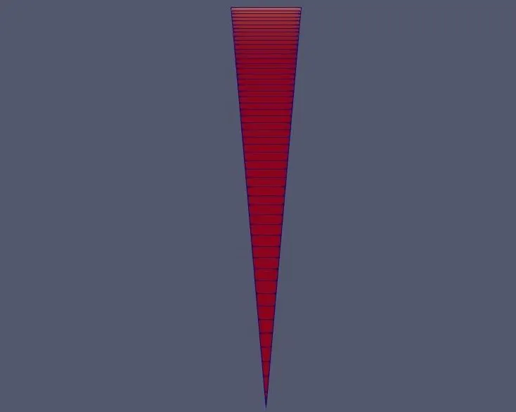
Mesh with 25 degrees:
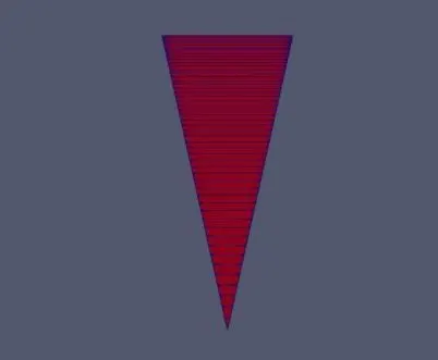
Mesh with 45 degreees:

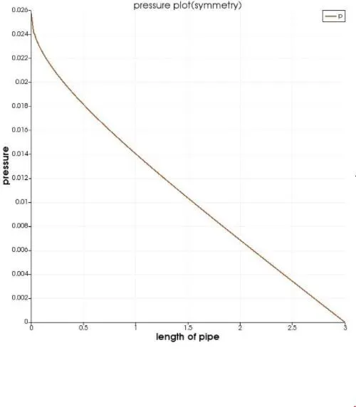
Symmetric boundary condition at 10 degrees:
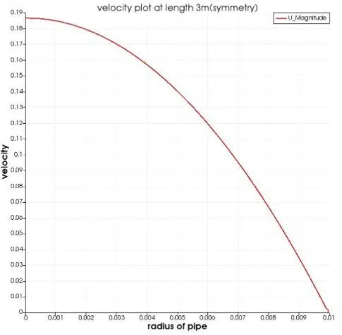
Pressure and velocity plots:
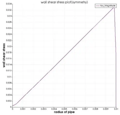
Wall shear stress plot:
1. The maximum velocity obtained from the openfoam is 0.186582 where as the analytical maximum velocity obtained from matlab is 0.1875, the error is 0.000918
2. The pressure drop obtained from openfoam is 0.025718 where as the analytical pressure drop obtained from matlab is 0.0201, the error is 0.005618
3. The maximum wall shear stress obtained from openfoam is 0.032909 where as the analytical maximum shear stress obtained from matlab is 0.0334, the error is 0.000491
Wedge boundary condition at 10 degrees:
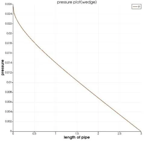
Pressure and velocity plots:
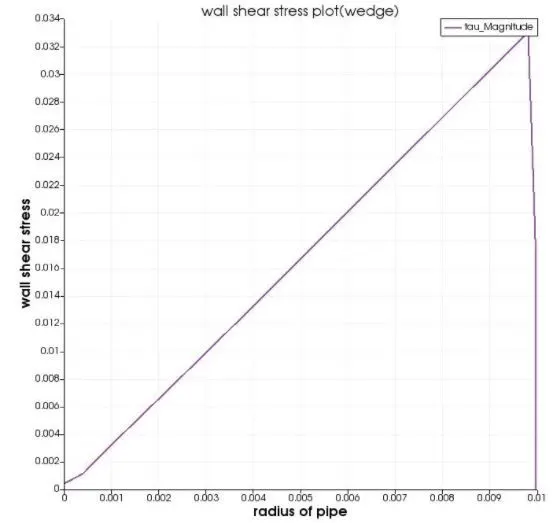
Wall shear stress plot:
1. The maximum velocity obtained from the openfoam is 0.186581 where as the analytical maximum velocity obtained from matlab is 0.1875, the error is 0.000919
2. The pressure drop obtained from openfoam is 0.0257238 where as the analytical pressure drop obtained from matlab is 0.0201, the error is 0.0056238
3. The maximum wall shear stress obtained from openfoam is 0.0329091 where as the analytical maximum shear stress obtained from matlab is 0.0334, the error is 0.000490
Symmetric boundary condition at 25 degrees:
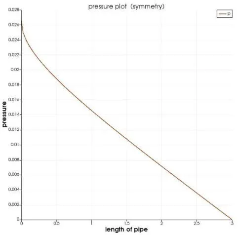
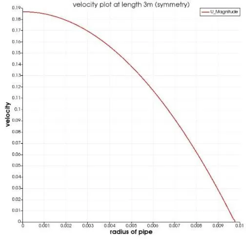
Pressure and velocity plot:
Wall shear stress plot:
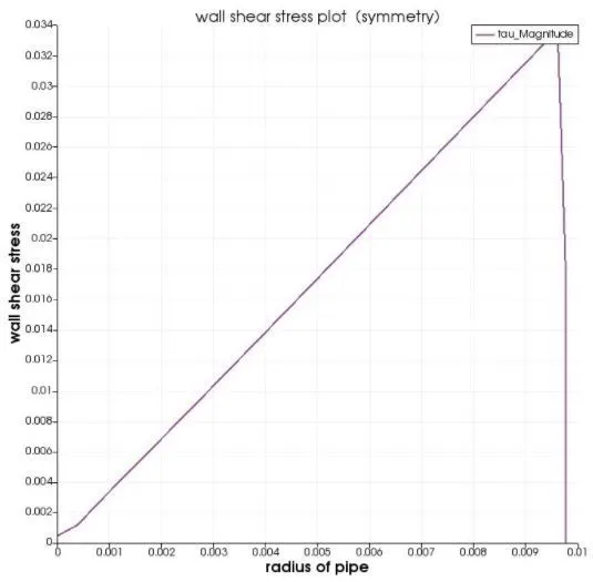
1. The maximum velocity obtained from the openfoam is 0.186692 where as the analytical maximum velocity obtained from matlab is 0.1875, the error is 0.000808
2. The pressure drop obtained from openfoam is 0.0265624 where as the analytical pressure drop obtained from matlab is 0.0201, the error is 0.0064624
3. The maximum wall shear stress obtained from openfoam is 0.0336332 where as the analytical maximum shear stress obtained from matlab is 0.0334, the error is 0.0002332
Wedge boundary condition at 25 degrees:
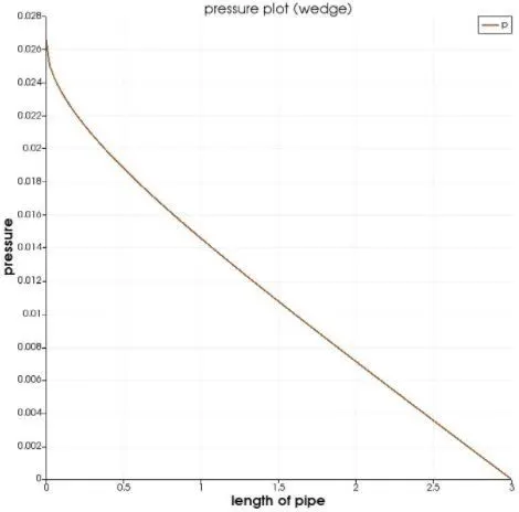
Pressure and velocity plot:
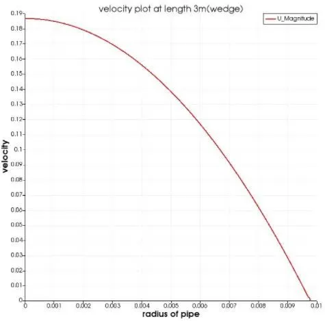
Wall shear stress plot:
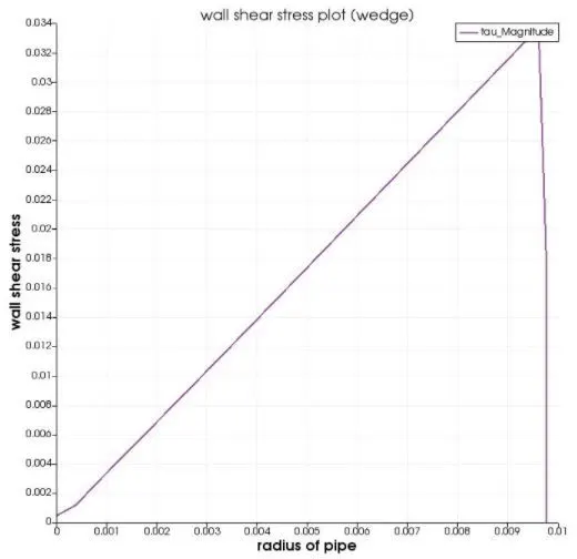
1. The maximum velocity obtained from the openfoam is 0.186692 where as the analytical maximum velocity obtained from matlab is 0.1875, the error is 0.000808
2. The pressure drop obtained from openfoam is 0.0265641 where as the analytical pressure drop obtained from matlab is 0.0201, the error is 0.0064641
3. The maximum wall shear stress obtained from openfoam is 0.0336332 where as the analytical maximum shear stress obtained from matlab is 0.0334, the error is 0.0002332
Symmetric boundary condition at 45 degrees:
Pressure and velocity plot:
Wall shear stress plot:
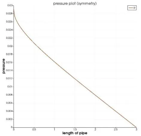
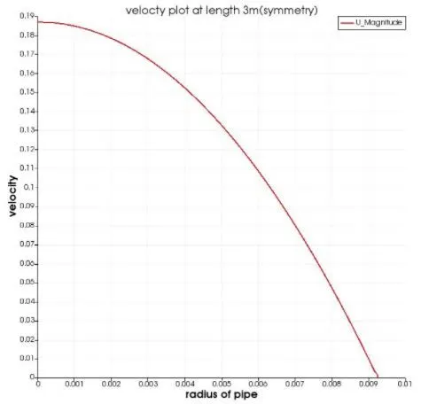
1. the maximum velocity obtained from the openfoam is 0.186919 where as the analytical maximum velocity obtained from matlab is 0.1875, the error is 0.000581
2. the pressure drop obtained from openfoam is 0.0290308 where as the analytical pressure drop obtained from matlab is 0.0201, the error is 0.0089308
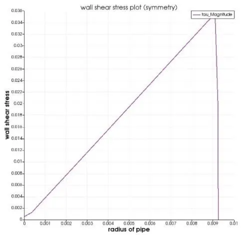
3. the maximum wall shear stress obtained from openfoam is 0.0352642 where as the analytical maximum shear stress obtained from matlab is 0.0334, the error is 0.0018642
Wedge boundary condition at 45 degrees:
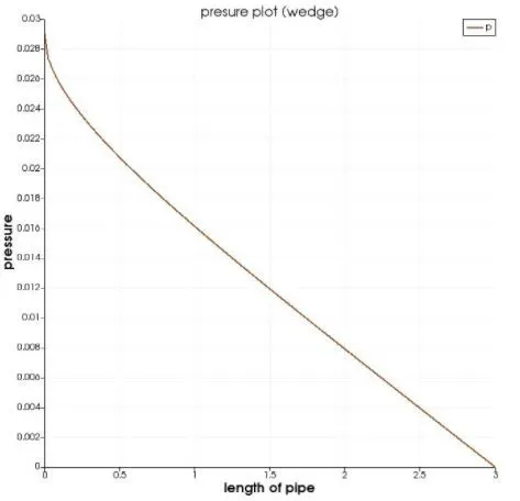
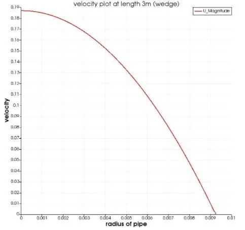
Pressure and velocity plot:
Wall shear stress plot:
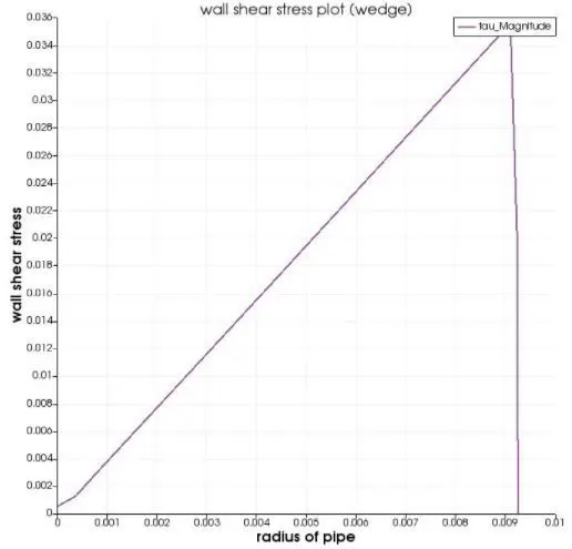
1. The maximum velocity obtained from the openfoam is 0.186919 where as the analytical maximum velocity obtained from matlab is 0.1875, the error is 0.000581
2. The pressure drop obtained from openfoam is 0.0290388 where as the analytical pressure drop obtained from matlab is 0.0201, the error is 0.0.0089388
3. The maximum wall shear stress obtained from openfoam is 0.0354713 where as the analytical maximum shear stress obtained from matlab is 0.0334, the error is 0.0020713.
CONCLUSION:
1. By comparing both the results with symmetric and wedge boundary conditions at 45 degrees, the error obtained using symmetric boundary condition is less compared with using of wedge boundary condition. but the error keeps on increaing with increasing angle from 25 to 45 degrees. with this we conclude that error in primitive variables increases with increase in angle.
2. With the increase of wedge angle, by using of symmetric boundary conditions the error in primitive variables is less compared to using of wedge boundary condition. the execution time for wedge boundary condition is higher compared to symmetric boundary condition.
3. with the increase in wedge angle, the error in maximum velocity gets decreased in both wedge and symmetric boundary conditions.
4. we can use symmetric boundary conditions for all the mirror planes, but we can use wedge boundary condition for only axi-symmetric planes.