Week 12 - Validation studies of Symmetry BC vs Wedge BC in OpenFOAM vs Analytical H.P equation
-
Point: To concentrate on the impact of the wedge point and the Limit Conditions on the reproduction of an axisymmetric laminar stream in a tube shaped pipe.
Hypothetical Presentation:
Axi-symmetric stream: A stream design is axisymmetric when indistinguishable in each plane goes through a specific straight-line. The straight-line being referred to is alluded to as the balance hub.
Each longitudinal plane through the pivot would show the equivalent smooth out design.Laminar Stream: In liquid elements, laminar stream is described by liquid particles following smooth ways in layers, with each layer moving flawlessly past the contiguous layers with practically no blending. At low speeds, the liquid will in general stream without sidelong blending, and contiguous layers slide past each other like playing a card game. There are no cross-flows opposite to the heading of stream, nor vortexes or twirls of liquids. In laminar stream, the liquid particles' movement is methodical, with particles near a strong surface moving in straight lines lined up with that surface.
Laminar stream is a stream system portrayed by high energy dispersion and low force convection.
At the point when a liquid moves through a shut channel like a line or between two level plates, both of two kinds of stream might happen relying upon the liquid's speed and thickness: laminar stream or violent stream. Laminar stream happens at lower speeds, under a limit at which the stream becomes violent. The not entirely settled by a dimensionless boundary describing the stream called the Reynolds number, which likewise relies upon the consistency and thickness of the liquid and aspects of the channel. 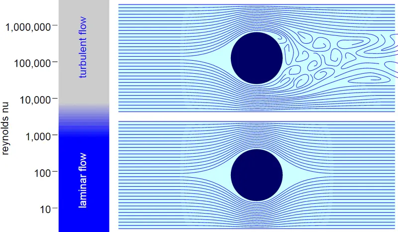
Comparison between Turbulent and Laminar Flow.
Reynolds Number: The Reynolds number (Re) predicts stream designs in various liquid stream circumstances. At low Reynolds numbers, streams will quite often be overwhelmed by laminar (sheet-like) stream, while at high Reynolds numbers, streams will generally be violent. The choppiness results from contrasts in the liquid's speed and course, which may in some cases cross or even move counter to the stream's general bearing (whirlpool ebbs and flows). These vortex flows start to beat the stream, spending energy simultaneously, which for fluids builds the possibilities of cavitation. Reynolds numbers are a significant dimensionless amount in liquid mechanics.
The Reynolds number has wide applications, going from fluid stream in a line to the section of air over an airplane wing. It is utilized to foresee the progress from laminar to violent stream and is utilized in the scaling of comparable yet unique estimated stream circumstances, for example, between an airplane model in an air stream and the standard variant. The expectations of the beginning of choppiness and the capacity to compute scaling impacts can be utilized to assist with foreseeing liquid conduct for a bigger scope, like in nearby or worldwide air or water development and in this manner the related meteorological and climatological impacts.Methodology:
1. The methodology for this challenge includes altering the recently made MATLAB code and changing the information and the Limit Conditions in OpenFoam.
2. In the Robotized BlockMeshDict document, we want to alter the wedge plot for one specific limit condition. The places where we are playing out the reproduction and afterward concentrating on the recreation results are:
The code for Wedge Boundary Condition at a wedge angle of 45 deg is as follows:
clear all
close all
clc

%Inputs:
l= 1.5;         %Length of the pipe.
theta = 45.0;    %Wedge angle.
d = 0.01;       %Diameter of the pipe.
c = 1.0;        %Conversion Factor.
r = d/2;        %Radius of the Cylinder.
nx = 500;       %number of Mesh points in x-direction on the block.
ny= 25;         %Number of Mesh points in the y-direction on the block.
nz= 1;          %number of Mesh Points in the z-direction on the block.
gx = 1;         %Grading along the x-direction.
gy = 1;         %Grading along the y-direction.
gz = 1;         %Grading along the z-direction.


f1 = fopen('BlockMeshDict.txt','w');
fprintf(f1,'/*--------------------------------*- C++ -*----------------------------------*n');
fprintf(f1,'  =========                 | n');
fprintf(f1,'        /  F ield         | OpenFOAM: The Open Source CFD Toolbox n');
fprintf(f1,'       /   O peration     | Website:  https://openfoam.org n');
fprintf(f1,'      /    A nd           | Version:  8 n');
fprintf(f1,'     /     M anipulation  | n');
fprintf(f1,'/*------------------------------------------------------------------*/ n');
fprintf(f1, 'FoamFile n');
fprintf(f1,'{ n');
fprintf(f1,'    version     2.0; n');
fprintf(f1,'    format      ascii; n' );
fprintf(f1,'    class       dictionary; n');
fprintf(f1,'    object      blockMeshDict; n');
fprintf(f1,'} n');
fprintf(f1,'// * * * * * * * * * * * * * * * * * * * * * * * * * * * * * * * * * * * * * // n');

fprintf(f1,'convertToMeters %0.1f; n',c);
fprintf(f1,'n');
fprintf(f1,'vertices n');
fprintf(f1,'( n');
fprintf(f1,'(0 0 0) n');
fprintf(f1,'(%0.6f %0.6f %0.3f)n',r*sind(theta/2),r*cosd(theta/2),0);
fprintf(f1, '(%0.6f %0.6f %0.3f)n',-r*sind(theta/2),r*cosd(theta/2),0);
fprintf(f1,'(0 0 %0.3f) n',-l);
fprintf(f1,'(%0.6f %0.6f %0.3f)n',r*sind(theta/2),r*cosd(theta/2),-l);
fprintf(f1, '(%0.6f %0.6f %0.3f)n',-r*sind(theta/2),r*cosd(theta/2),-l);
fprintf(f1,'); n');
fprintf(f1,'n');

fprintf(f1,'blocks n');
fprintf(f1,'( n');
fprintf(f1,'hex (0 3 5 2 0 3 4 1) (%0.0f %0.0f %0.0f) simpleGrading (%0.0f %0.0f %0.0f) n',nx,ny,nz,gx,gy,gz);
fprintf(f1,'); n');
fprintf(f1,'n');

fprintf(f1,'edges n');
fprintf(f1,'( n');
fprintf(f1,'); n');
fprintf(f1,'n');

fprintf(f1,'boundary n');
fprintf(f1,'( n');
fprintf(f1,'in n');
fprintf(f1,'{ n');
fprintf(f1,'type patch; n');
fprintf(f1,'faces n');
fprintf(f1,'( n');
fprintf(f1,'(0 1 2 0) n');
fprintf(f1,'); n');
fprintf(f1,'} n');

fprintf(f1,'out n');
fprintf(f1,'{ n');
fprintf(f1,'type patch; n');
fprintf(f1,'faces n');
fprintf(f1,'( n');
fprintf(f1,'(3 5 4 3) n');
fprintf(f1,'); n');
fprintf(f1,'} n');

fprintf(f1,'ft n');
fprintf(f1,'{ n');
fprintf(f1,'type wedge; n');
fprintf(f1,'faces n');
fprintf(f1,'( n');
fprintf(f1,'(0 3 4 1) n');
fprintf(f1,'); n');
fprintf(f1,'} n');

fprintf(f1,'bk n');
fprintf(f1,'{ n');
fprintf(f1,'type wedge; n');
fprintf(f1,'faces n');
fprintf(f1,'( n');
fprintf(f1,'(3 0 2 5) n');
fprintf(f1,'); n');
fprintf(f1,'} n');

fprintf(f1,'top n');
fprintf(f1,'{ n');
fprintf(f1,'type wall; n');
fprintf(f1,'faces n');
fprintf(f1,'( n');
fprintf(f1,'(5 2 1 4) n');
fprintf(f1,'); n');
fprintf(f1,'} n');

fprintf(f1,'axis n');
fprintf(f1,'{ n');
fprintf(f1,'type empty; n');
fprintf(f1,'faces n');
fprintf(f1,'( n');
fprintf(f1,'(0 3 3 0) n');
fprintf(f1,'); n');
fprintf(f1, '} n');

fprintf(f1,'); n');
fprintf(f1,'n');

fprintf(f1,'mergePatchPairs n');
fprintf(f1,'( n');
fprintf(f1,'); n');
fprintf(f1,'n');
fprintf(f1,'// ************************************************************************* // n');


%END
The code for Symmetry Boundary Condition at a wedge angle of 45 deg is as follows:
clear all
close all
clc

%Inputs:
l= 1.5;         %Length of the pipe.
theta = 45.0;    %Wedge angle.
d = 0.01;       %Diameter of the pipe.
c = 1.0;        %Conversion Factor.
r = d/2;        %Radius of the Cylinder.
nx = 500;       %number of Mesh points in x-direction on the block.
ny= 25;         %Number of Mesh points in the y-direction on the block.
nz= 3;          %number of Mesh Points in the z-direction on the block.
gx = 1;         %Grading along the x-direction.
gy = 1;         %Grading along the y-direction.
gz = 1;         %Grading along the z-direction.


f1 = fopen('BlockMeshDict.txt','w');
fprintf(f1,'/*--------------------------------*- C++ -*----------------------------------*n');
fprintf(f1,'  =========                 | n');
fprintf(f1,'        /  F ield         | OpenFOAM: The Open Source CFD Toolbox n');
fprintf(f1,'       /   O peration     | Website:  https://openfoam.org n');
fprintf(f1,'      /    A nd           | Version:  8 n');
fprintf(f1,'     /     M anipulation  | n');
fprintf(f1,'/*------------------------------------------------------------------*/ n');
fprintf(f1, 'FoamFile n');
fprintf(f1,'{ n');
fprintf(f1,'    version     2.0; n');
fprintf(f1,'    format      ascii; n' );
fprintf(f1,'    class       dictionary; n');
fprintf(f1,'    object      blockMeshDict; n');
fprintf(f1,'} n');
fprintf(f1,'// * * * * * * * * * * * * * * * * * * * * * * * * * * * * * * * * * * * * * // n');

fprintf(f1,'convertToMeters %0.1f; n',c);
fprintf(f1,'n');
fprintf(f1,'vertices n');
fprintf(f1,'( n');
fprintf(f1,'(0 0 0) n');
fprintf(f1,'(%0.6f %0.6f %0.3f)n',r*sind(theta/2),r*cosd(theta/2),0);
fprintf(f1, '(%0.6f %0.6f %0.3f)n',-r*sind(theta/2),r*cosd(theta/2),0);
fprintf(f1,'(0 0 %0.3f) n',-l);
fprintf(f1,'(%0.6f %0.6f %0.3f)n',r*sind(theta/2),r*cosd(theta/2),-l);
fprintf(f1, '(%0.6f %0.6f %0.3f)n',-r*sind(theta/2),r*cosd(theta/2),-l);
fprintf(f1,'); n');
fprintf(f1,'n');

fprintf(f1,'blocks n');
fprintf(f1,'( n');
fprintf(f1,'hex (0 3 5 2 0 3 4 1) (%0.0f %0.0f %0.0f) simpleGrading (%0.0f %0.0f %0.0f) n',nx,ny,nz,gx,gy,gz);
fprintf(f1,'); n');
fprintf(f1,'n');

fprintf(f1,'edges n');
fprintf(f1,'( n');
fprintf(f1,'); n');
fprintf(f1,'n');

fprintf(f1,'boundary n');
fprintf(f1,'( n');
fprintf(f1,'in n');
fprintf(f1,'{ n');
fprintf(f1,'type patch; n');
fprintf(f1,'faces n');
fprintf(f1,'( n');
fprintf(f1,'(0 1 2 0) n');
fprintf(f1,'); n');
fprintf(f1,'} n');

fprintf(f1,'out n');
fprintf(f1,'{ n');
fprintf(f1,'type patch; n');
fprintf(f1,'faces n');
fprintf(f1,'( n');
fprintf(f1,'(3 5 4 3) n');
fprintf(f1,'); n');
fprintf(f1,'} n');

fprintf(f1,'ft n');
fprintf(f1,'{ n');
fprintf(f1,'type symmetry; n');
fprintf(f1,'faces n');
fprintf(f1,'( n');
fprintf(f1,'(0 3 4 1) n');
fprintf(f1,'); n');
fprintf(f1,'} n');

fprintf(f1,'bk n');
fprintf(f1,'{ n');
fprintf(f1,'type symmetry; n');
fprintf(f1,'faces n');
fprintf(f1,'( n');
fprintf(f1,'(3 0 2 5) n');
fprintf(f1,'); n');
fprintf(f1,'} n');

fprintf(f1,'top n');
fprintf(f1,'{ n');
fprintf(f1,'type wall; n');
fprintf(f1,'faces n');
fprintf(f1,'( n');
fprintf(f1,'(5 2 1 4) n');
fprintf(f1,'); n');
fprintf(f1,'} n');

fprintf(f1,'axis n');
fprintf(f1,'{ n');
fprintf(f1,'type empty; n');
fprintf(f1,'faces n');
fprintf(f1,'( n');
fprintf(f1,'(0 3 3 0) n');
fprintf(f1,'); n');
fprintf(f1, '} n');

fprintf(f1,'); n');
fprintf(f1,'n');

fprintf(f1,'mergePatchPairs n');
fprintf(f1,'( n');
fprintf(f1,'); n');
fprintf(f1,'n');
fprintf(f1,'// ************************************************************************* // n');


%END
3. So, we must run the simulation and plot the necessary graphs at all the Boundary Conditions' angles, i.e. Wedge Boundary conditions and the Symmetry Boundary Condition. We must make use of the plot over line command to study how the shear force is varying with a change in the distance along the radial direction. In contrast, the Pressure drop is to be studied in the fully developed region along the Axial Direction.
To plot the line, we must use the plot over line command. This will help us study the data variation along that line.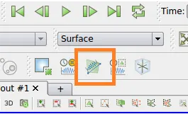
Then, we must plot the co-ordinates along which we want to study the data. Here, we need to properly give the coordinates as they will determine the plot and the data we study.
The coordinates are given as follows: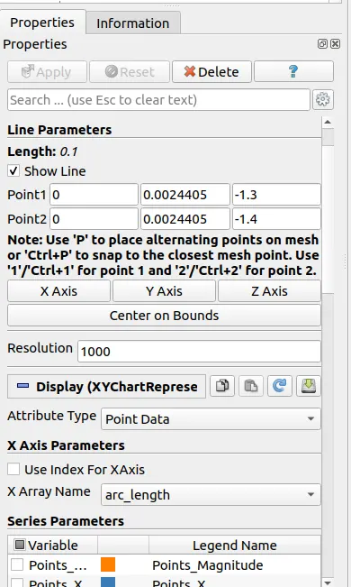
The line is drawn, as shown below: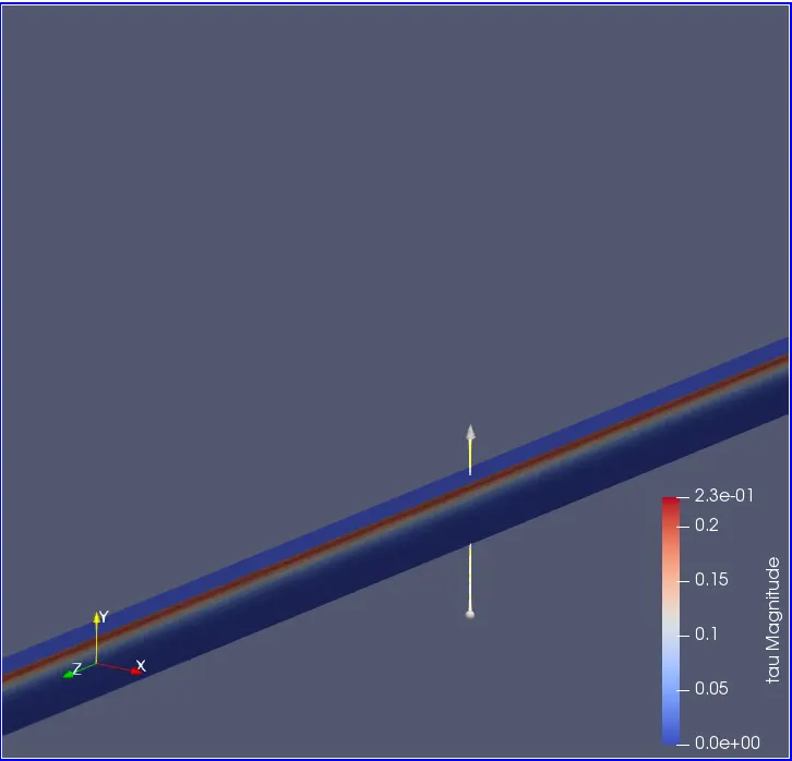
4. We must change the Boundary condition for this and then run the simulation for the same angles. Another location where we need to change is the Initial Conditions. For the wedge's front and Back faces, we must specify the condition as Symmetry instead of Wedge.
5. After all the simulations were run, the results are to be compared and then findings are to be studied.- Result:
1. The first simulation comparison is with the Wedge Boundary condition. Within this Boundary Condition, the simulation comparison for all the above-mentioned angles is as follows.
We will compare the Shear Stress developed for both the boundary conditions at all three angles.
a.Shear Stress Variation with respect to the Radial Distance.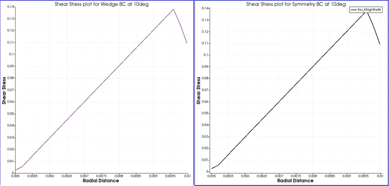
The Shear Stress plot for both the Boundary Conditions, the wedge Boundary Condition and the Symmetry Boundary Condition are shown at 10degrees. We can see that when we apply the Symmetry Boundary Condition, the slope of the curve is much higher than when we apply the Wedge Boundary Condition. So, when we apply the Symmetry Boundary Condition, the Mesh becomes 3D, and the computation is done for all three global axes. This affects the calculation as well. The peak value in the Wedge Boundary Condition is approximately 0.145 units, but whereas when we apply the Symmetry Boundary Condition, the peak value touches around 0.140units.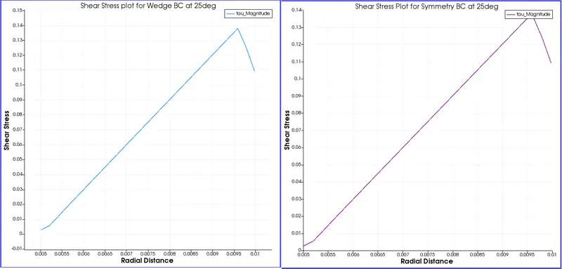
The graph shown above is comparing the Shear Stress for both the boundary conditions for when the wedge angle is 25degrees.
Similarly, we plot and study all the graphs, as shown below: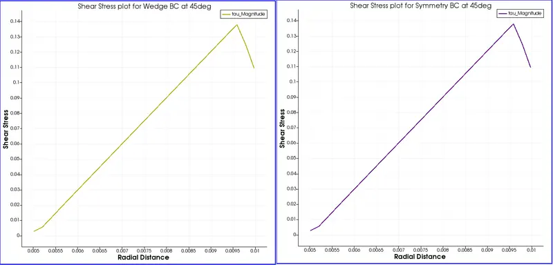
This graph compares the Shear Stress at 45 Deg for both the Boundary conditions.
b. Velocity Variation with respect to Radial Distance.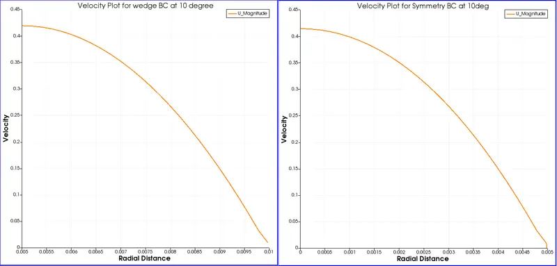
Velocity variation at 10degrees for the two Boundary Conditions.
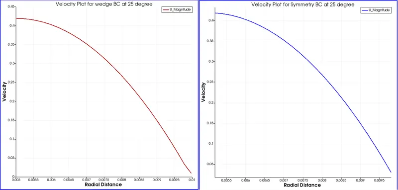
Velocity variation at 25 degrees for the two Boundary Conditions.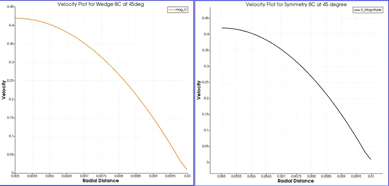
Velocity variation at 45 degrees for the two Boundary Conditions.
c. Pressure Drop across the axial Distance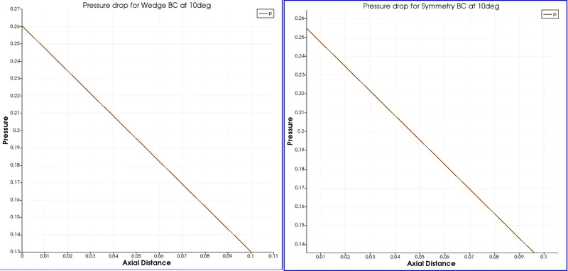
Pressure drop at 10 degrees across the Axial Distance.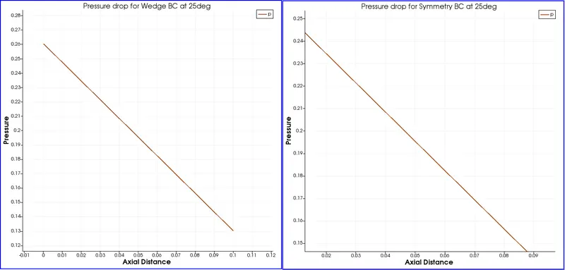
Pressure drop at 25 degrees across the Axial Distance.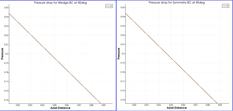
Pressure drop at 45 degrees across the Axial Distance. - Validation:
a.Validation of Maximum Pressure drop in the Fully developed Region.
These graphs depict the change in the various parameters for both the Boundary Conditions, and we can compare these quantities properly.
Like for example, we can compare the pressure drop from the graph and the pressure drop that we get analytically.
From the graph, we can see that the maximum value - minimum value = 0.26 - 0.13 = 0.13units = 130Pascal.
And, when we calculate it analytically, we know that the formula is :
For a Kinematic Viscosity of 1.924e-5(Used in the simulation), the Dynamic Viscosity is 1.924e-5*1000 = 1.924e-2units.
Calculating using these values, we get= 0.129units = 129Pascal.
The error between the Analytical value and the value obtained from the graph is (0.13-0.129) / (0.129) = 0.7%, which is under the tolerance limit of 5%.
Now, because the error is under tolerance, we can conclude that the simulation has reached a Steady State.
b.Validation of the Maximum Velocity
Now, if we wish to compare the Maximum velocity from the graph, we can see that the value is 0.42units.
According to the Analytical formula, we know that the maximum velocity must be:
And our Vavg is 0.21units; hence the analytical value will be 0.42units that matches the value that we get from the graph.
c. To validate the Hydrodynamic length with the Numerical Result.
So, In fluid dynamics, the entrance length is the distance a flow travels after entering a pipe before the flow becomes fully developed. Entrance length refers to the length of the entry region, the area following the pipe entrance where effects originating from the interior wall of the pipe propagate into the flow as an expanding boundary layer.
Here, numerically, we know that the velocity profile will be different before and after the Hydrodynamic entry length. After the Hydrodynamic entry length, the Velocity profile will be the final parabolic profile that it must have in a fully developed region.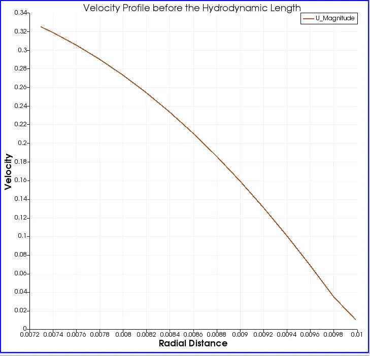
Velocity profile before the Hydrodynamic Length
Here is the velocity profile before the Hydrodynamic Length. We can see that this plot is not properly parabolic.
The location where the velocity was measured for the above plot: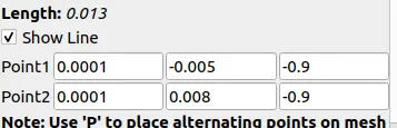
Whereas, if we compare the velocity profile at a location after the hydrodynamic length and in the fully developed region, the velocity profile will be much more defined and proper.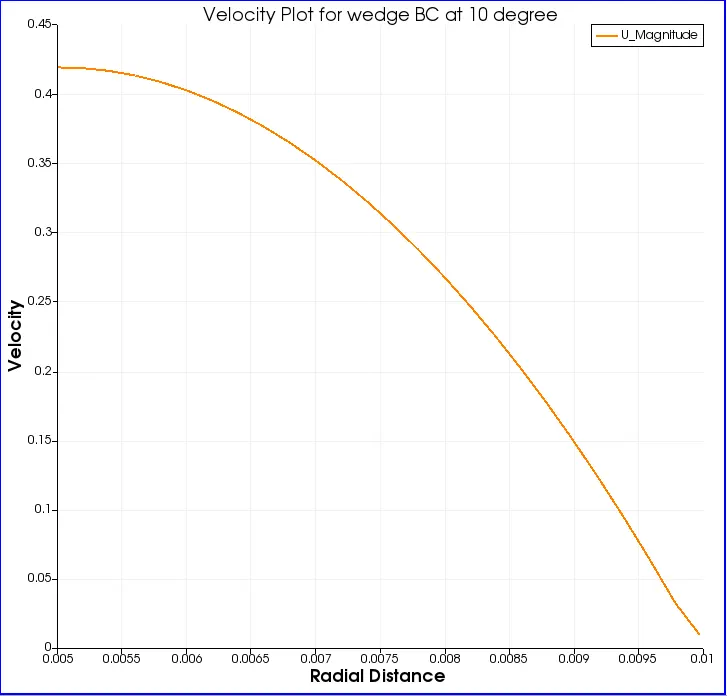
Velocity after the Hydrodynamic length
The location where the velocity was measured for the above plot: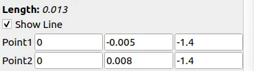
Now, If we wish to calculate the Hydrodynamic length analytically, the formula is as follows:
where:
Re = Reynolds number.
D = Diameter.
In our case, Re = 2100 and the Diameter = 0.1m, so the Hydrodynamic Length is:
Lh = 0.005*2100*0.1 = 1.05m.
And from the two graphs above, we can confirm that only after the Hydrodynamic length of approximately 1.0m, the velocity profile is changing into a fully parabolic shape.
d. Shear Stress Plot: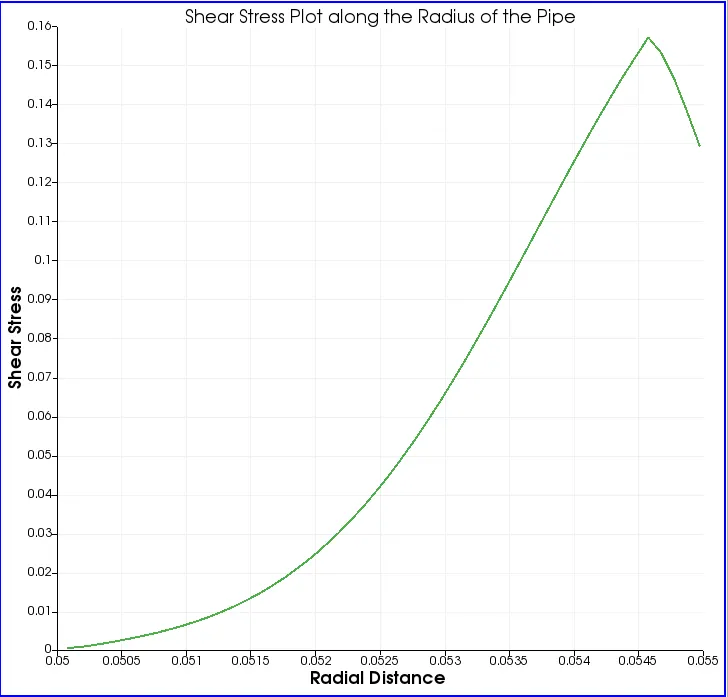
Shear Stress Plot
Shear Stress is the maximum near the wall because of the friction that the wall has. But, as we move away from the wall, the Shear Force decreases, and it can be confirmed with the graph above.
According to the Analytically calculated profile, the graph is:
And we know that this profile also gives out a Parabolic curve similar to the one we have gotten in the graph.
e. Comparison between the two Boundary Conditions.
We have performed Simulation for two Boundary Conditions; those are Symmetry Boundary Condition and the Wedge Boundary Condition.
During the Wedge Boundary condition simulation, the simulation across the arc of the wedge is not done, but whereas in the case of Symmetry Boundary Condition, the calculation across the arc of the wedge is done; hence the simulation time is higher in that case. The Courant number is increasing slightly in the case of wedge Boundary Condition and hence the Symmetry Boundary Condition will be slightly more accurate. The Symmetry Boundary condition considers the Mesh as 3D and the calculation is done along all the three global axes.
We understand the results should not change due to the change in the Boundary conditions, and this is because the Physics of the problem does not change and remains the same.
Conclusion: In conclusion, I would like to state that this challenge helped me understand the difference between the two boundary conditions and how to simulate them as per the need of the problem that we will be simulating.