Week 12 - Validation studies of Symmetry BC vs Wedge BC in OpenFOAM vs Analytical H.P equation
VALIDATION STUDIES OF SYMMETRY BC VS WEDGE BC IN OpenFOAM VS ANALYTICAL H.P. EQUATION
ABSTRACT:
- The flow through a pipe is the case of internal flow.
- Their major application is in the refrigeration and air conditioning industries.
- The fluid velocity is zero at the walls and maximum at the center.
- In fluid flow, it is preferred to take average velocity because it remains constant when the flow is incompressible Laminar and the cross-sectional area of the pipe is constant.
Assumptions:
- The steady laminar incompressible flow of a fluid is taken.
- There is no velocity in the radial direction.
- There is no acceleration since the flow is steady.
- Reynolds number for the laminar flow is 2100.
- Only the wedge shape of the pipe is considered because the flow is axis-symmetric.
- The equation governing the fluid flow is described by the Hagen-Poiseuille equation.
Entrance length:
The length of the entrance is the distance that fluid travels after entering a pipe before the full development of the flow. Entrance length refers to the length of the entry region, where effects from the pipe's interior wall spread as an expanding boundary layer into the flow.
Hydrodynamic entrance length (L_h):
The hydrodynamic entrance region refers to the area of a pipe where fluid entering a pipe develops a velocity profile due to viscous forces spreading from a pipe's interior wall. This region has a non-uniform flow. The fluid enters a pipe at a constant speed, so fluid particles in the layer in contact with the pipe's surface come to a complete stop because of the no-slip rule. The layer in contact with the pipe surface is resistant to the acceleration of neighboring layers due to viscous forces within the fluid and slowly slows down adjacent layers of fluid, creating a velocity profile.
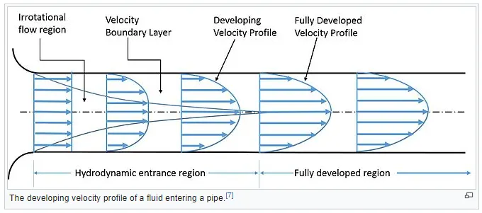
To keep the mass true, the speed of the fluid layers in the center of the pipe increases to compensate for the reduced speed of the fluid layers near the surface of the pipe. It creates a gradient of velocity across the pipe cross-section. Hydrodynamically fully developed region means u = u(r). The length of the hydrodynamic entry region along the pipe is called the hydrodynamic entry length. It is a function of the Reynolds Number of the flow. In the case of laminar flow, this length is given by:

Where,
Re - is the Reynolds number
D - is the diameter of the pipe.
Hagen-Poiseuille Equation:
The assumptions of the equations are that the fluid is incompressible and Newtonian, the flow is laminar through a pipe of a constant cross-section of length that is longer than the diameter, and there is no acceleration of the fluid in the pipe. The velocity profile remains unchanged in the hydrodynamically fully developed region, and the shear stress at the wall also remains unchanged.
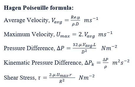
Observations based on the Hagen-Poiseuille equation
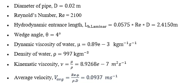
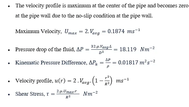
PROCEDURE:
1. The procedure for this challenge involves editing the previously made MATLAB code and changing the input angle and the Boundary Conditions in both MATLAB and OpenFoam.
2. In the Automated BlockMeshDict file, we need to run the code for both boundary conditions for each of the following wedge angles,
a. `10^0`
b. `25^0`
c. `45^0`
3. Then, we must run the simulation and plot the necessary graphs at all the Boundary Conditions angles(i.e. Wedge Boundary conditions and the Symmetry Boundary Condition).
4. We must change the Boundary conditions type from wedge to symmetry for the front and the back walls in the following files,
- In MATLAB code.
- In OpenFOAM, cavity>0>p
- In OpenFOAM, cavity>0>U
5. After all the simulations were run, the results are to be compared, and then the findings are to be studied.
MATLAB Code:
Below MATLAB codes will generate the mesh file (blockMeshDict file) for OpenFOAM. The geometry used is a wedge made out of a single block and for different wedge angles, these MATLAB programs create the required blockMeshDict file.
1)Wedge BC code for wedge angle `10^0`
% simulation of a flow in a pipe
clear all
close all
clc

% defining input values from Hagen Poiseuille
% Reynolds number for laminar flow
Re = 2100;

% diameter of pipe (m)
D = 0.02;

% radius of pipe (m)
R = D/2;

% wedge angle
thetha = 10;

% dynamic viscosity of water (pa.s)
mu = 0.89e-3;

% density of water (kg/m^3)
rho = 997;

% kinematic viscosity (m^2/s)
nu = mu/rho;

% hydrodynamic entry length (m)
L_h = 0.0575*Re*D;
fprintf("hydrodynamic entrance length, L_h = %.4f m \n",L_h);

% assumed characteristic length (m)
L = L_h+0.3;
fprintf("\nAssumed length of pipe, L = %.4f m \n",L);

% calculating average velocity (m/s)
v_avg = (Re*nu)/D;

% calculating maximum velocity at the centerline of pipe (m/s)
u_max = 2*v_avg;

% darcy friction factor
f = 4/Re;

% pressure drop for the laminar flow (N/m^2)
% the pressure drop is for fully developed profile as taken L > L_h
delta_p = (32*mu*v_avg*L)/D^2;
fprintf("\nStatic Pressure Drop for fully developed flow, p_s = %.4f n/m^2\n",delta_p);


%% Vertices co-ordinate
v0 = [0 0 0];                                %point 0
v1 = [0 R*cosd(thetha/2) -R*sind(thetha/2)]; %point 1
v2 = [0 R*cosd(thetha/2) R*sind(thetha/2)];  %point 2
v3 = [L 0 0];                                %point 3
v4 = [L R*cosd(thetha/2) -R*sind(thetha/2)]; %point 4
v5 = [L R*cosd(thetha/2) R*sind(thetha/2)];  %point 5


%% writing the script for blockMeshDict file
% creating file with permission to write
f1 = fopen('blockMeshDict.txt','w');

%headers
h1 = ("/*--------------------------------*- C++ -*----------------------------------*\");
h2 = ("  =========                 |");
h3 = ("  \\      /  F ield         | OpenFOAM: The Open Source CFD Toolbox");
h4 = ("   \\    /   O peration     | Website:  https://openfoam.org");
h5 = ("    \\  /    A nd           | Version:  10");
h6 = ("     \\/     M anipulation  |");
h7 = ("\*---------------------------------------------------------------------------*/");

h8 = ("FoamFile");
h9 = ("{");
h10 = ("    format      ascii;");
h11 = ("    class       dictionary;");
h12 = ("    object      blockMeshDict;");
h13 = ("}");
h14 = ("// * * * * * * * * * * * * * * * * * * * * * * * * * * * * * * * * * * * * * //");

h16 = ("convertToMeters 1;");

%comment lines
fprintf(f1,"%s\n",h1);
fprintf(f1,"%s\n",h2);
fprintf(f1,"%s\n",h3);
fprintf(f1,"%s\n",h4);
fprintf(f1,"%s\n",h5);
fprintf(f1,"%s\n",h6);
fprintf(f1,"%s\n",h7);

%file identifiers
fprintf(f1,"%s\n",h8);
fprintf(f1,"%s\n",h9);
fprintf(f1,"%s\n",h10);
fprintf(f1,"%s\n",h11);
fprintf(f1,"%s\n",h12);
fprintf(f1,"%s\n",h13);
fprintf(f1,"%s\n\n",h14);

%scaling factor
fprintf(f1,"%s\n\n",h16);

%vertices
fprintf(f1,"vertices\n");
fprintf(f1,"(\n");
fprintf(f1,"\t(%d %d %d)\n",v0);
fprintf(f1,"\t(%d %d %d)\n",v1);
fprintf(f1,"\t(%d %d %d)\n",v2);
fprintf(f1,"\t(%d %d %d)\n",v3);
fprintf(f1,"\t(%d %d %d)\n",v4);
fprintf(f1,"\t(%d %d %d)\n",v5);
fprintf(f1,");\n\n");

%blocks
fprintf(f1,"blocks\n");
fprintf(f1,"(\n");
%number of mesh points and grading factor can be varied using below line
fprintf(f1,"\thex (0 1 2 0 3 4 5 3) (50 1 200) simpleGrading (0.4 1 1)\n");
fprintf(f1,");\n\n");

%edges
fprintf(f1,"edges\n");
fprintf(f1,"(\n");
fprintf(f1,"\tarc 1 2 (0 %4.2f 0)\n",R);
fprintf(f1,"\tarc 4 5 (%4.2f %4.2f 0)\n",L,R);
fprintf(f1,");\n\n");

%boundary
fprintf(f1,"boundary\n");
fprintf(f1,"(\n");

fprintf(f1,"\taxis \n");
fprintf(f1,"\t{ \n");
fprintf(f1,"\t  type empty; \n");
fprintf(f1,"\t  faces \n");
fprintf(f1,"\t  ( \n");
fprintf(f1,"\t\t(0 3 3 0)\n");
fprintf(f1,"\t  );\n");
fprintf(f1,"\t}\n");

fprintf(f1,"\tinlet \n");
fprintf(f1,"\t{ \n");
fprintf(f1,"\t  type patch; \n");
fprintf(f1,"\t  faces \n");
fprintf(f1,"\t  ( \n");
fprintf(f1,"\t\t(0 0 2 1)\n");
fprintf(f1,"\t  );\n");
fprintf(f1,"\t}\n");

fprintf(f1,"\tpipe_surface \n");
fprintf(f1,"\t{ \n");
fprintf(f1,"\t  type wall; \n");
fprintf(f1,"\t  faces \n");
fprintf(f1,"\t  ( \n");
fprintf(f1,"\t\t(1 4 5 2)\n");
fprintf(f1,"\t  );\n");
fprintf(f1,"\t}\n");

fprintf(f1,"\toutlet \n");
fprintf(f1,"\t{ \n");
fprintf(f1,"\t  type patch; \n");
fprintf(f1,"\t  faces \n");
fprintf(f1,"\t  ( \n");
fprintf(f1,"\t\t(3 4 5 3)\n");
fprintf(f1,"\t  );\n");
fprintf(f1,"\t}\n");

fprintf(f1,"\tfront \n");
fprintf(f1,"\t{ \n");
fprintf(f1,"\t  type wedge; \n");
fprintf(f1,"\t  faces \n");
fprintf(f1,"\t  ( \n");
fprintf(f1,"\t\t(0 3 5 2)\n");
fprintf(f1,"\t  );\n");
fprintf(f1,"\t}\n");

fprintf(f1,"\tback \n");
fprintf(f1,"\t{ \n");
fprintf(f1,"\t  type wedge; \n");
fprintf(f1,"\t  faces \n");
fprintf(f1,"\t  ( \n");
fprintf(f1,"\t\t(0 1 4 3)\n");
fprintf(f1,"\t  );\n");
fprintf(f1,"\t}\n");

fprintf(f1,");\n\n");
fprintf(f1,"mergePatchPairs\n");
fprintf(f1,"(\n");
fprintf(f1,");\n\n");
fprintf(f1,"// * * * * * * * * * * * * * * * * * * * * * * * * * * * * * * * * * * * * * //\n");


%% shear stress and velocity profile

% diameter of the pipe is 0.02 m
%radius of the pipe is 0.01 m

r = linspace(-0.01,0.01,100);

for i=1:length(r)
    tau(i)=(2*mu*u_max*abs(r(i))) / R^2;
    u(i) = 2*v_avg*(1-(r(i)^2/R^2));
end

%plots
%Shear stress plot
figure(1)
plot(tau,r ,'linewidth',2)
grid on
xlabel('Shear stress in Pascal')
ylabel('Radius of pipe in Meter')
title('Shear stress profile (analytical method)')
legend('Shear stress profile')

%veloctiy profile
figure(2)
plot(u,r ,'linewidth',2)
grid on
xlabel('Velocity in m/s')
ylabel('Radius of pipe in Meter')
title('Velocity profile (analytical method)')
legend('velocity profile (fully developed flow)')

%values to be displayed

v_max_analytic = max(u);
p_k = delta_p / rho;     %kinematic pressure m^2/s^2

fprintf("\nKinematic Pressure Drop for fully developed flow, p_k = %.4f m^2/s^2\n",p_k);
fprintf("\nAverage velocity using HP equation, V_avg = %.4f m/s \n",v_avg);
fprintf("\nMaximum velocity using HP equation, u_max = %.4f m/s \n",u_max);
fprintf("\nMaximum velocity using analytic method, u_max = %.4f m/s \n",v_max_analytic);
2)Symmetry BC code for wedge angle `10^0`
% simulation of a flow in a pipe
clear all
close all
clc

% defining input values from Hagen Poiseuille
% Reynolds number for laminar flow
Re = 2100;

% diameter of pipe (m)
D = 0.02;

% radius of pipe (m)
R = D/2;

% wedge angle
thetha = 10;

% dynamic viscosity of water (pa.s)
mu = 0.89e-3;

% density of water (kg/m^3)
rho = 997;

% kinematic viscosity (m^2/s)
nu = mu/rho;

% hydrodynamic entry length (m)
L_h = 0.0575*Re*D;
fprintf("hydrodynamic entrance length, L_h = %.4f m \n",L_h);

% assumed characteristic length (m)
L = L_h+0.3;
fprintf("\nAssumed length of pipe, L = %.4f m \n",L);

% calculating average velocity (m/s)
v_avg = (Re*nu)/D;

% calculating maximum velocity at the centerline of pipe (m/s)
u_max = 2*v_avg;

% darcy friction factor
f = 4/Re;

% pressure drop for the laminar flow (N/m^2)
% the pressure drop is for fully developed profile as taken L > L_h
delta_p = (32*mu*v_avg*L)/D^2;
fprintf("\nStatic Pressure Drop for fully developed flow, p_s = %.4f n/m^2\n",delta_p);


%% Vertices co-ordinate
v0 = [0 0 0];                                %point 0
v1 = [0 R*cosd(thetha/2) -R*sind(thetha/2)]; %point 1
v2 = [0 R*cosd(thetha/2) R*sind(thetha/2)];  %point 2
v3 = [L 0 0];                                %point 3
v4 = [L R*cosd(thetha/2) -R*sind(thetha/2)]; %point 4
v5 = [L R*cosd(thetha/2) R*sind(thetha/2)];  %point 5


%% writing the script for blockMeshDict file
% creating file with permission to write
f1 = fopen('blockMeshDict.txt','w');

%headers
h1 = ("/*--------------------------------*- C++ -*----------------------------------*\");
h2 = ("  =========                 |");
h3 = ("  \\      /  F ield         | OpenFOAM: The Open Source CFD Toolbox");
h4 = ("   \\    /   O peration     | Website:  https://openfoam.org");
h5 = ("    \\  /    A nd           | Version:  10");
h6 = ("     \\/     M anipulation  |");
h7 = ("\*---------------------------------------------------------------------------*/");

h8 = ("FoamFile");
h9 = ("{");
h10 = ("    format      ascii;");
h11 = ("    class       dictionary;");
h12 = ("    object      blockMeshDict;");
h13 = ("}");
h14 = ("// * * * * * * * * * * * * * * * * * * * * * * * * * * * * * * * * * * * * * //");

h16 = ("convertToMeters 1;");

%comment lines
fprintf(f1,"%s\n",h1);
fprintf(f1,"%s\n",h2);
fprintf(f1,"%s\n",h3);
fprintf(f1,"%s\n",h4);
fprintf(f1,"%s\n",h5);
fprintf(f1,"%s\n",h6);
fprintf(f1,"%s\n",h7);

%file identifiers
fprintf(f1,"%s\n",h8);
fprintf(f1,"%s\n",h9);
fprintf(f1,"%s\n",h10);
fprintf(f1,"%s\n",h11);
fprintf(f1,"%s\n",h12);
fprintf(f1,"%s\n",h13);
fprintf(f1,"%s\n\n",h14);

%scaling factor
fprintf(f1,"%s\n\n",h16);

%vertices
fprintf(f1,"vertices\n");
fprintf(f1,"(\n");
fprintf(f1,"\t(%d %d %d)\n",v0);
fprintf(f1,"\t(%d %d %d)\n",v1);
fprintf(f1,"\t(%d %d %d)\n",v2);
fprintf(f1,"\t(%d %d %d)\n",v3);
fprintf(f1,"\t(%d %d %d)\n",v4);
fprintf(f1,"\t(%d %d %d)\n",v5);
fprintf(f1,");\n\n");

%blocks
fprintf(f1,"blocks\n");
fprintf(f1,"(\n");
%number of mesh points and grading factor can be varied using below line
fprintf(f1,"\thex (0 1 2 0 3 4 5 3) (50 1 200) simpleGrading (0.4 1 1)\n");
fprintf(f1,");\n\n");

%edges
fprintf(f1,"edges\n");
fprintf(f1,"(\n");
fprintf(f1,"\tarc 1 2 (0 %4.2f 0)\n",R);
fprintf(f1,"\tarc 4 5 (%4.2f %4.2f 0)\n",L,R);
fprintf(f1,");\n\n");

%boundary
fprintf(f1,"boundary\n");
fprintf(f1,"(\n");

fprintf(f1,"\taxis \n");
fprintf(f1,"\t{ \n");
fprintf(f1,"\t  type empty; \n");
fprintf(f1,"\t  faces \n");
fprintf(f1,"\t  ( \n");
fprintf(f1,"\t\t(0 3 3 0)\n");
fprintf(f1,"\t  );\n");
fprintf(f1,"\t}\n");

fprintf(f1,"\tinlet \n");
fprintf(f1,"\t{ \n");
fprintf(f1,"\t  type patch; \n");
fprintf(f1,"\t  faces \n");
fprintf(f1,"\t  ( \n");
fprintf(f1,"\t\t(0 0 2 1)\n");
fprintf(f1,"\t  );\n");
fprintf(f1,"\t}\n");

fprintf(f1,"\tpipe_surface \n");
fprintf(f1,"\t{ \n");
fprintf(f1,"\t  type wall; \n");
fprintf(f1,"\t  faces \n");
fprintf(f1,"\t  ( \n");
fprintf(f1,"\t\t(1 4 5 2)\n");
fprintf(f1,"\t  );\n");
fprintf(f1,"\t}\n");

fprintf(f1,"\toutlet \n");
fprintf(f1,"\t{ \n");
fprintf(f1,"\t  type patch; \n");
fprintf(f1,"\t  faces \n");
fprintf(f1,"\t  ( \n");
fprintf(f1,"\t\t(3 4 5 3)\n");
fprintf(f1,"\t  );\n");
fprintf(f1,"\t}\n");

fprintf(f1,"\tfront \n");
fprintf(f1,"\t{ \n");
fprintf(f1,"\t  type symmetry; \n");
fprintf(f1,"\t  faces \n");
fprintf(f1,"\t  ( \n");
fprintf(f1,"\t\t(0 3 5 2)\n");
fprintf(f1,"\t  );\n");
fprintf(f1,"\t}\n");

fprintf(f1,"\tback \n");
fprintf(f1,"\t{ \n");
fprintf(f1,"\t  type symmetry; \n");
fprintf(f1,"\t  faces \n");
fprintf(f1,"\t  ( \n");
fprintf(f1,"\t\t(0 1 4 3)\n");
fprintf(f1,"\t  );\n");
fprintf(f1,"\t}\n");

fprintf(f1,");\n\n");
fprintf(f1,"mergePatchPairs\n");
fprintf(f1,"(\n");
fprintf(f1,");\n\n");
fprintf(f1,"// * * * * * * * * * * * * * * * * * * * * * * * * * * * * * * * * * * * * * //\n");


%% shear stress and velocity profile

% diameter of the pipe is 0.02 m
%radius of the pipe is 0.01 m

r = linspace(-0.01,0.01,100);

for i=1:length(r)
    tau(i)=(2*mu*u_max*abs(r(i))) / R^2;
    u(i) = 2*v_avg*(1-(r(i)^2/R^2));
end

%plots
%Shear stress plot
figure(1)
plot(tau,r ,'linewidth',2)
grid on
xlabel('Shear stress in Pascal')
ylabel('Radius of pipe in Meter')
title('Shear stress profile (analytical method)')
legend('Shear stress profile')

%veloctiy profile
figure(2)
plot(u,r ,'linewidth',2)
grid on
xlabel('Velocity in m/s')
ylabel('Radius of pipe in Meter')
title('Velocity profile (analytical method)')
legend('velocity profile (fully developed flow)')

%values to be displayed

v_max_analytic = max(u);
p_k = delta_p / rho;     %kinematic pressure m^2/s^2

fprintf("\nKinematic Pressure Drop for fully developed flow, p_k = %.4f m^2/s^2\n",p_k);
fprintf("\nAverage velocity using HP equation, V_avg = %.4f m/s \n",v_avg);
fprintf("\nMaximum velocity using HP equation, u_max = %.4f m/s \n",u_max);
fprintf("\nMaximum velocity using analytic method, u_max = %.4f m/s \n",v_max_analytic);- In above codes 1 and 2, change the wedge angle input to `25^0` and `45^0` to generate the required blockMeshDict files.
Symmetry BC code for wedge angle `10^0` (sample for understanding)
BlockMeshDict:
/*--------------------------------*- C++ -*----------------------------------*\
  =========                 |
  \\      /  F ield         | OpenFOAM: The Open Source CFD Toolbox
   \\    /   O peration     | Website:  https://openfoam.org
    \\  /    A nd           | Version:  10
     \\/     M anipulation  |
\*---------------------------------------------------------------------------*/
FoamFile
{
    format      ascii;
    class       dictionary;
    object      blockMeshDict;
}
// * * * * * * * * * * * * * * * * * * * * * * * * * * * * * * * * * * * * * //

convertToMeters 1;

vertices
(
	(0 0 0)
	(0 9.961947e-03 -8.715574e-04)
	(0 9.961947e-03 8.715574e-04)
	(2.715000e+00 0 0)
	(2.715000e+00 9.961947e-03 -8.715574e-04)
	(2.715000e+00 9.961947e-03 8.715574e-04)
);

blocks
(
	hex (0 1 2 0 3 4 5 3) (50 1 200) simpleGrading (0.4 1 1)
);

edges
(
	arc 1 2 (0 0.01 0)
	arc 4 5 (2.71 0.01 0)
);

boundary
(
	axis
	{
	  type empty;
	  faces
	  (
		(0 3 3 0)
	  );
	}
	inlet
	{
	  type patch;
	  faces
	  (
		(0 0 2 1)
	  );
	}
	pipe_surface
	{
	  type wall;
	  faces
	  (
		(1 4 5 2)
	  );
	}
	outlet
	{
	  type patch;
	  faces
	  (
		(3 4 5 3)
	  );
	}
	front
	{
	  type symmetry;
	  faces
	  (
		(0 3 5 2)
	  );
	}
	back
	{
	  type symmetry;
	  faces
	  (
		(0 1 4 3)
	  );
	}
);

mergePatchPairs
(
);

// * * * * * * * * * * * * * * * * * * * * * * * * * * * * * * * * * * * * * //
ControlDict:
/*--------------------------------*- C++ -*----------------------------------*\
  =========                 |
  \\      /  F ield         | OpenFOAM: The Open Source CFD Toolbox
   \\    /   O peration     | Website:  https://openfoam.org
    \\  /    A nd           | Version:  10
     \\/     M anipulation  |
\*---------------------------------------------------------------------------*/
FoamFile
{
    format      ascii;
    class       dictionary;
    location    "system";
    object      controlDict;
}
// * * * * * * * * * * * * * * * * * * * * * * * * * * * * * * * * * * * * * //

application     icoFoam;

startFrom       startTime;

startTime       0;

stopAt          endTime;

endTime         10;

deltaT          0.01;

writeControl    timeStep;

writeInterval   10;

purgeWrite      0;

writeFormat     ascii;

writePrecision  6;

writeCompression off;

timeFormat      general;

timePrecision   6;

runTimeModifiable true;


// ************************************************************************* //
Initial conditions - Kinematic pressure drop:
/*--------------------------------*- C++ -*----------------------------------*\
  =========                 |
  \\      /  F ield         | OpenFOAM: The Open Source CFD Toolbox
   \\    /   O peration     | Website:  https://openfoam.org
    \\  /    A nd           | Version:  10
     \\/     M anipulation  |
\*---------------------------------------------------------------------------*/
FoamFile
{
    format      ascii;
    class       volScalarField;
    object      p;
}
// * * * * * * * * * * * * * * * * * * * * * * * * * * * * * * * * * * * * * //

dimensions      [0 2 -2 0 0 0 0];

internalField   uniform 0;

boundaryField
{
    axis
    {
        type            empty;
    }

    inlet
    {
        type            zeroGradient;
    }

    pipe_surface
    {
        type            zeroGradient;
    }

    outlet
    {
         type           fixedValue;
         value          uniform 0.0182;
    }

    front
    {
         type            symmetry;
    }

    back
    {
         type            symmetry;
    }

}

// ************************************************************************* //
Initial conditions -Inlet Average velocity:
/*--------------------------------*- C++ -*----------------------------------*
  =========                 |
  \      /  F ield         | OpenFOAM: The Open Source CFD Toolbox
   \    /   O peration     | Website:  https://openfoam.org
    \  /    A nd           | Version:  8
     \/     M anipulation  |
*---------------------------------------------------------------------------*/
FoamFile
{
    version     2.0;
    format      ascii;
    class       volVectorField;
    object      U;
}
// * * * * * * * * * * * * * * * * * * * * * * * * * * * * * * * * * * * * * //

dimensions      [0 1 -1 0 0 0 0];

internalField   uniform (0.0937 0 0);

boundaryField
{
    axis
    {
        type            empty;

    }
    inlet
    {
        type            fixedValue;
        value           uniform (0.0937 0 0);
    }
    pipe_surface
    {
        type            fixedValue;
        value           uniform (0 0 0);

    }

    outlet
    {
        type            zeroGradient;

    }
    front
    {
         type            symmetry;
    }
    back
    {
         type            symmetry;
    }

}

// ************************************************************************* //
Transport Properties- Kinematic viscosity:
/*--------------------------------*- C++ -*----------------------------------*\
  =========                 |
  \\      /  F ield         | OpenFOAM: The Open Source CFD Toolbox
   \\    /   O peration     | Website:  https://openfoam.org
    \\  /    A nd           | Version:  10
     \\/     M anipulation  |
\*---------------------------------------------------------------------------*/
FoamFile
{
    format      ascii;
    class       dictionary;
    location    "constant";
    object      physicalProperties;
}
// * * * * * * * * * * * * * * * * * * * * * * * * * * * * * * * * * * * * * //

nu              [0 2 -1 0 0 0 0] 8.9268e-07;


// ************************************************************************* //
OUTPUTS:
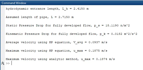
1) some of the MATLAB values which are useful for OpenFOAM simulation,
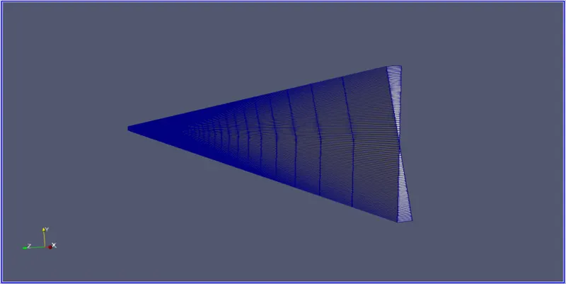
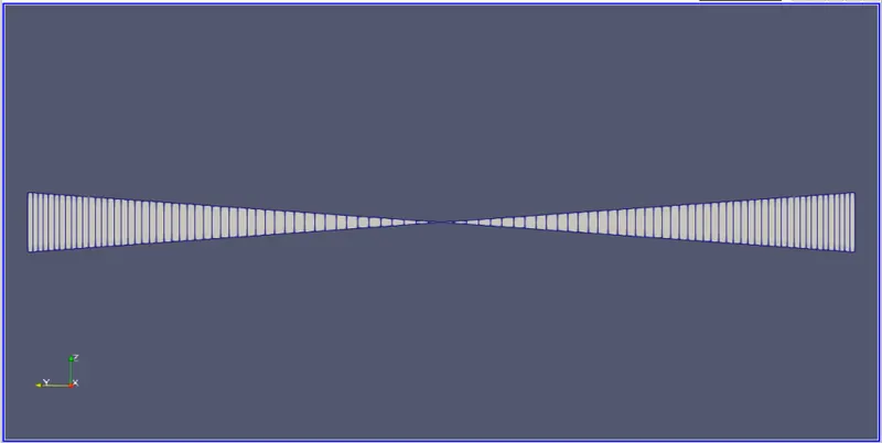
2) The wedge generated using MATLAB and OpenFOAM is reflected along Y-axis for better understanding and plot generation
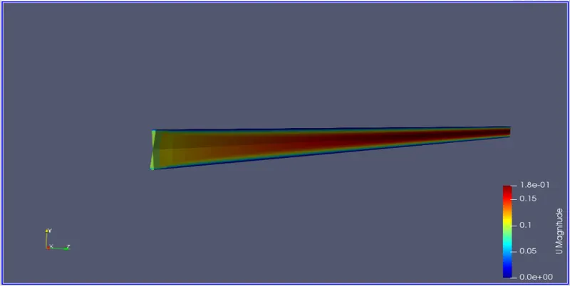
3) The velocity profile at the final timestep of the laminar incompressible flow of fluid through a pipe of a constant cross-section,
4) The Pressure profile at the final timestep of the laminar incompressible flow of fluid through a pipe of a constant cross-section,
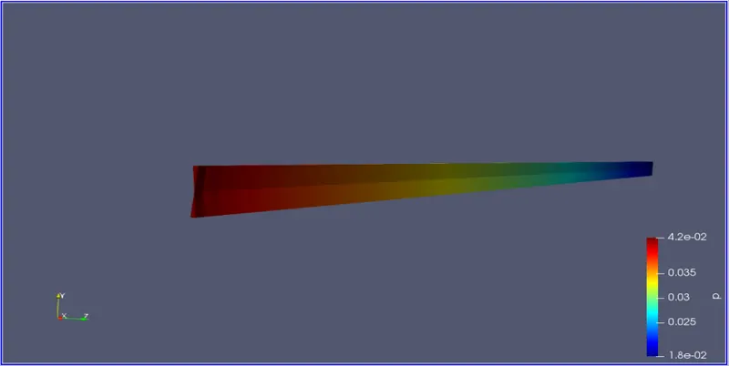
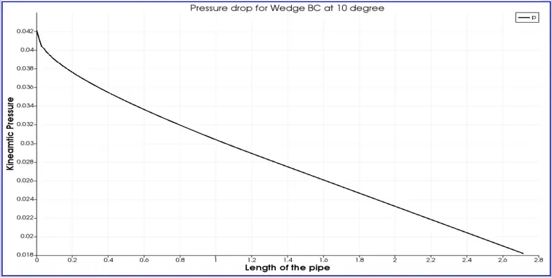
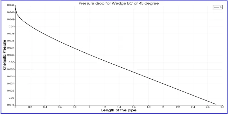
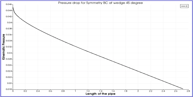
5) ParaView plots representing Pressure flow through the length of the pipe for different wedge angles and BC,
a) wedge angle = `10^0`
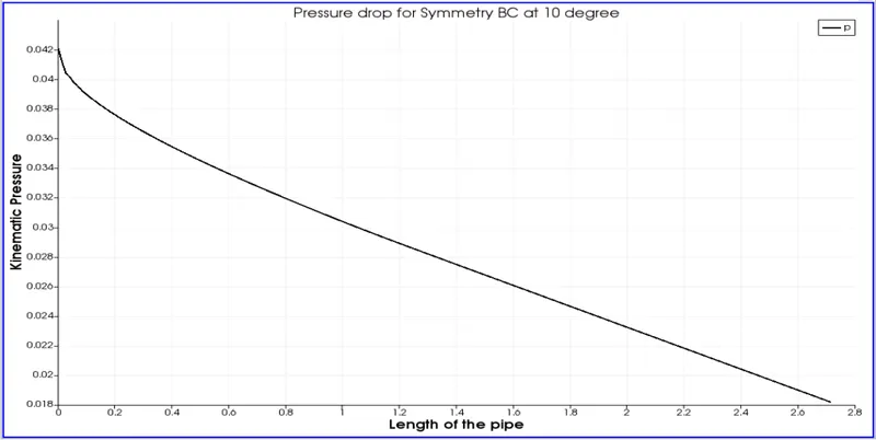
b) wedge angle = `25^0`
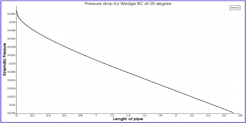
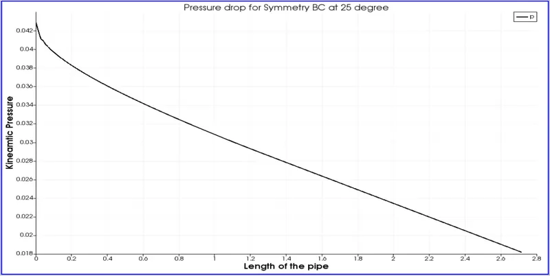
c) wedge angle = `45^0`
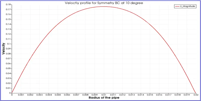
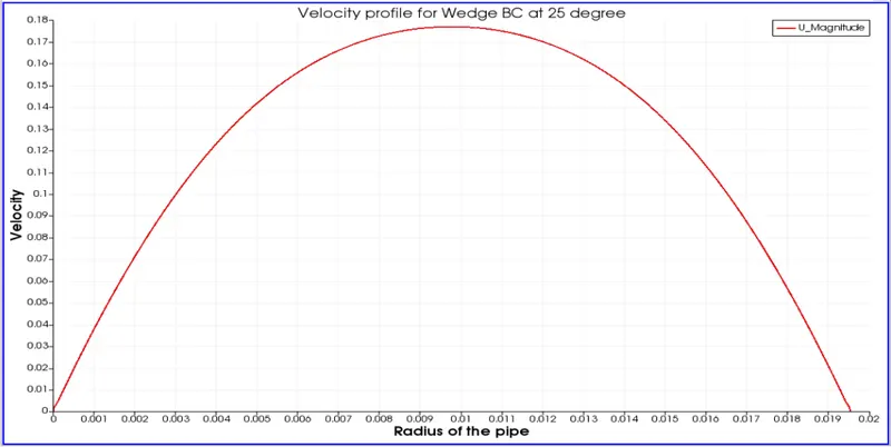
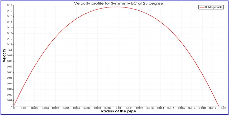
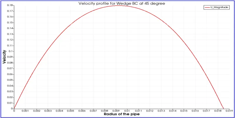
6) ParaView plots representing the Velocity profile of a fully developed flow (hydrodynamic entrance length, L =2.415 m) for different wedge angles and BC,
a) wedge angle = `10^0`
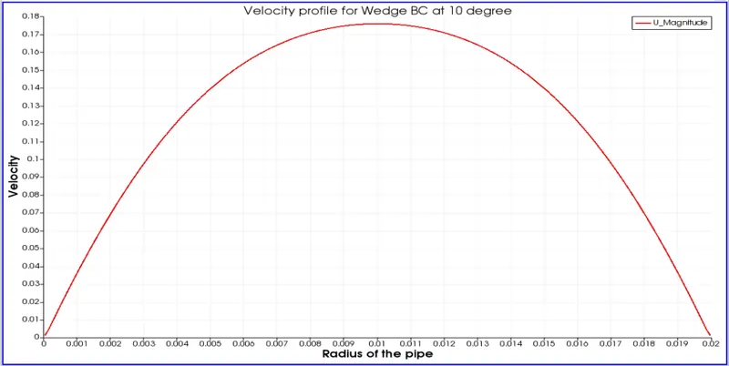
b) wedge angle = `25^0`
c) wedge angle = `45^0`
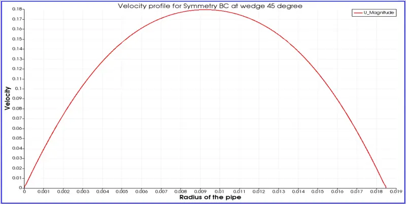
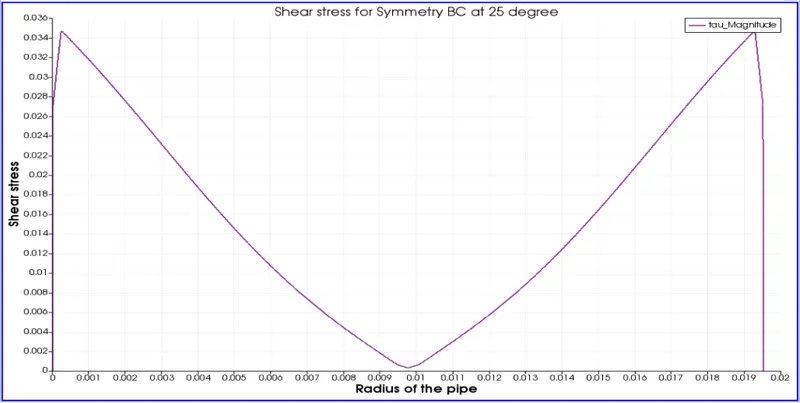
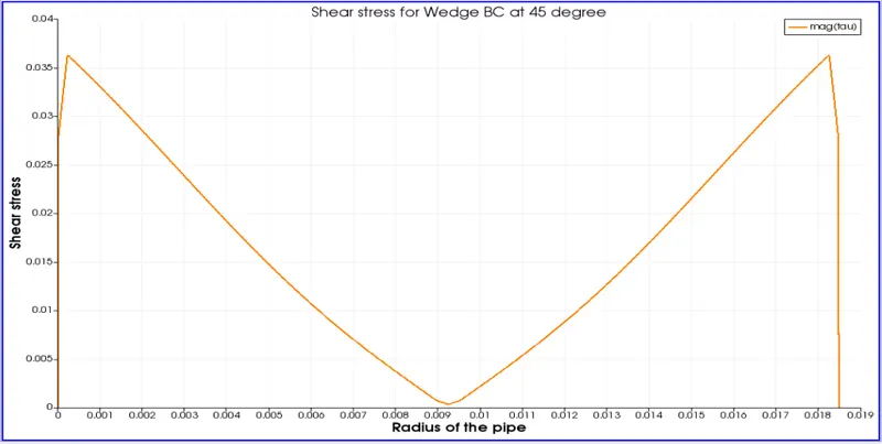
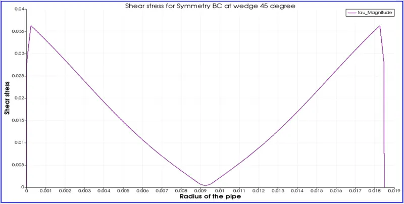
7) ParaView plots representing the Shear stress profile for different wedge angles and BC,
a) wedge angle = `10^0`
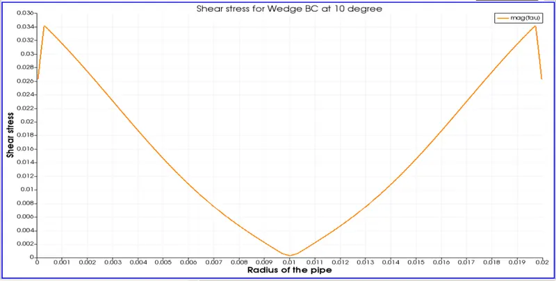
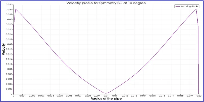
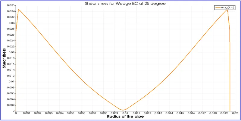
b) wedge angle = `25^0`
c) wedge angle = `45^0`
OBSERVATION:
1) Pressure:
- The pressure drop can be observed from the plot.
- As the fluid travels through the pipe from the inlet to the outlet, its pressure starts to drop gradually.
2) Velocity:
- The velocity profile is plotted at varying distances from the inlet (L=0 m) of the pipe.
- At the inlet (L=0 m), the velocity remains uniform as there is no disturbance.
- The velocity at a distance L = 0.2 m and L = 0.5 m, from the inlet seems to be slow and stable around the center of the pipe which shows that the velocity is gradually developing. It suddenly becomes zero at the wall because of the no-slip condition. This region is called the hydrodynamic entrance region.
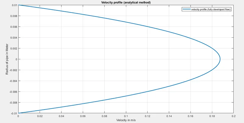
- The velocity profile at a distance of L = 2.5 m and L = 2.715 m is parabolic in nature because the velocity profile moves to the hydrodynamically fully developed region.
- Comparison of plots generated using MATLAB with OpenFOAM for wedge angle 10 and symmetry BC are shown below,
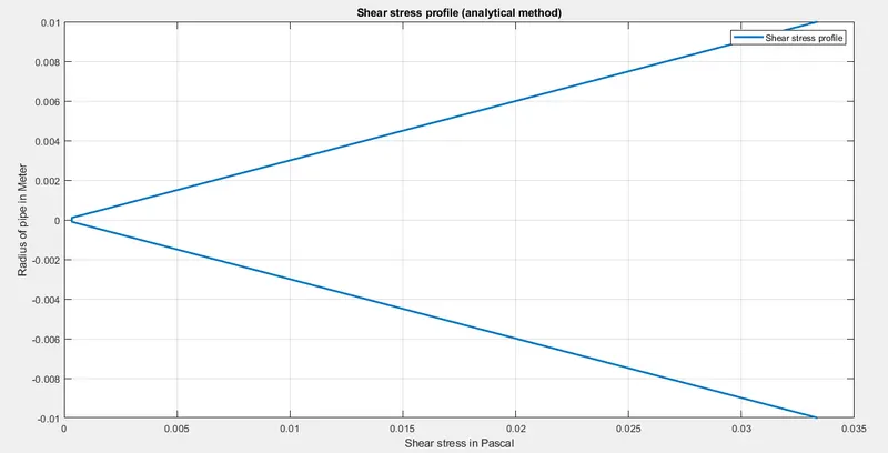
3)Shear stress:
- Shear Force is normally present because the adjacent layer of the fluid move with different velocities compared to each other.
- The irregularities can be observed in the shear stress profile because of the "finite volume method". At nodes intersection the value of shear stress increases, this can be reduced by increasing the number of grid points at the center of the pipe.
- The shear stress is maximum at the walls and is zero at the center of the pipe.
- Comparison of plots generated using MATLAB with OpenFOAM for wedge angle 25 and symmetry BC are shown below,
4)Comparison between the Boundary Conditions:
- We have performed a Simulation for the Symmetry Boundary Condition and the Wedge Boundary Condition.
- The Courant number is increasing slightly in the case of the wedge Boundary Condition and hence the Symmetry Boundary Condition will be slightly more accurate for complex problems.
- The Symmetry Boundary condition considers the Mesh as 3D and the calculation is done along all three global axes.
RESULT:
- The Hydrodynamic length (L_h) was found using MATLAB code and a fully developed flow velocity profile was obtained at the same length in the numerical method. Thus the hydrodynamic length is similar for both methods.
- The fully developed flow velocity profile was found to be similar for both analytical and numerical methods.
- The pressure drop for the fully developed flow is plotted and the maximum velocity of the fully developed flow,
for the analytical method, U_max = 0.1875 m/s
for the numerical method, U_max ~ 0.1765 m/s (from the plot)
- The above stats show that the velocity profile calculated numerically was equal to the HP equation with an error of 0.011 m/s.
- The post-process Shear stress was found and plotted using MATLAB.
- The wall shear stress for fully developed flow was plotted using ParaFOAM.
Differences observed between the symmetric and wedge boundary conditions are:
- The execution time for the symmetry boundary conditions is higher compared to the wedge boundary condition for this problem.
- The symmetric boundary conditions can be used for all the mirror plane problems, but the wedge boundary conditions are only suited for axis-symmetric planes.
- Finally, with the increase in wedge angle, the error in maximum velocity gets decreased in both wedge and symmetric boundary conditions.
- For axisymmetric flow cases, Wedge BC is preferred over symmetric BC.
REFERENCE:
- https://en.wikipedia.org/wiki/Entrance_length_(fluid_dynamics)
- https://www.openfoam.com/documentation/user-guide/4-mesh-generation-and-conversion/4.2-boundaries
- https://www.youtube.com/watch?v=nRXYWNEulio
- https://www.simscale.com/docs/simulation-setup/boundary-conditions/wedge/#:~:text=The%20wedge%20boundary%20condition%20is,given%20radius%20for%20all%20angles.
- https://www.simscale.com/docs/simulation-setup/boundary-conditions/symmetry/