Week 12 - Validation studies of Symmetry BC vs Wedge BC in OpenFOAM vs Analytical H.P equation
** Laminar Flow Through Pipe
A) For angle 10
pipe radius= 2cm, Raynold's number= 2100
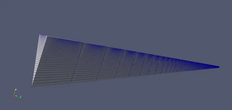
# Generating blockMeshDict file using MATLAB
FoamFile
{
	version     2.0;
	format      ascii;
	class       dictionary;
	object      blockMeshDict;
}
//******************************//
scale 1;
vertices
(
	(0 0 0)
	(0 0.019924 0.001743)
	(0 0.019924 -0.001743)
	(6.040000 0 0)
	(6.040000 0.019924 0.001743)
	(6.040000 0.019924 -0.001743)
);
blocks
(
hex (0 3 5 2 0 3 4 1) (150 40 1) simpleGrading (1 0.1 1)
);
edges
(
arc 1 2 (0 0.020000 0)
arc 4 5 (6.040000 0.020000 0)
);
boundary
(
	 inlet
	 {
		 type patch;
		 faces
		 (
			(0 1 2 0)
		 );
	 }
	 outlet
	 {
		 type patch;
		 faces
		 (
			(3 5 4 3)
		 );
	 }
	 front
	 {
		 type symmetry;
		 faces
		 (
			(0 3 4 1)
		 );
	 }
	 back
	 {
		 type symmetry;
		 faces
		 (
			(0 2 5 3)
		 );
	 }
	 axis
	 {
		 type empty;
		 faces
		 (
			(0 3 3 0)
		 );
	 }
	 pipeWall
	 {
		 type wall;
		 faces
		 (
			(1 4 5 2)
		 );
	 }
);
mergePatchPairs
(
);
//******************************//
Comment: The type of boundary for front and back is changed from wedge to symmetry.
The simulation time is calculated as: ntime=Lt/V
Lt=Entrance Length+1;
Velocity (v) is calculated from Raynold's number
v= Re*mu/(Rho*diameter)
Rho=1000; mu=8.9e-4
v=0.0467 m/s
# Editing 0 files
i) U file
/*--------------------------------*- C++ -*----------------------------------*\
| =========                 |                                                 |
| \\      /  F ield         | OpenFOAM: The Open Source CFD Toolbox           |
|  \\    /   O peration     | Version:  v2012                                 |
|   \\  /    A nd           | Website:  www.openfoam.com                      |
|    \\/     M anipulation  |                                                 |
\*---------------------------------------------------------------------------*/
FoamFile
{
    version     2.0;
    format      ascii;
    class       volVectorField;
    object      U;
}
// * * * * * * * * * * * * * * * * * * * * * * * * * * * * * * * * * * * * * //

dimensions      [0 1 -1 0 0 0 0];

internalField   uniform (0 0 0);

boundaryField
{
    inlet
    {
        type            fixedValue;
        value           uniform (0.046725 0 0);
    }

    outlet
    {
        type            zeroGradient;
    }

    front
    {
        type            symmetry;
    }

	back
    {
        type            symmetry;
    }

	axis
    {
        type            empty;
    }

	pipeWall
    {
        type            noSlip;
    }
}

// ************************************************************************* //
ii) p file
/*--------------------------------*- C++ -*----------------------------------*\
| =========                 |                                                 |
| \\      /  F ield         | OpenFOAM: The Open Source CFD Toolbox           |
|  \\    /   O peration     | Version:  v2012                                 |
|   \\  /    A nd           | Website:  www.openfoam.com                      |
|    \\/     M anipulation  |                                                 |
\*---------------------------------------------------------------------------*/
FoamFile
{
    version     2.0;
    format      ascii;
    class       volScalarField;
    object      p;
}
// * * * * * * * * * * * * * * * * * * * * * * * * * * * * * * * * * * * * * //

dimensions      [0 2 -2 0 0 0 0];

internalField   uniform 0;

boundaryField
{
    inlet
    {
        type            zeroGradient;
    }

	outlet
    {
        type            fixedValue;
		value           uniform 0;
    }

	front
    {
        type            symmetry;
    }

	back
    {
        type            s;
    }

	axis
    {
        type            empty;
    }

	pipeWall
    {
        type            zeroGradient;
    }

}

// ************************************************************************* //
# Editing transport properties file
/*--------------------------------*- C++ -*----------------------------------*\
| =========                 |                                                 |
| \\      /  F ield         | OpenFOAM: The Open Source CFD Toolbox           |
|  \\    /   O peration     | Version:  v2012                                 |
|   \\  /    A nd           | Website:  www.openfoam.com                      |
|    \\/     M anipulation  |                                                 |
\*---------------------------------------------------------------------------*/
FoamFile
{
    version     2.0;
    format      ascii;
    class       dictionary;
    location    "constant";
    object      transportProperties;
}
// * * * * * * * * * * * * * * * * * * * * * * * * * * * * * * * * * * * * * //

nu              8.7e-7;


// ************************************************************************* //
# Editing controlDict file
/*--------------------------------*- C++ -*----------------------------------*\
| =========                 |                                                 |
| \\      /  F ield         | OpenFOAM: The Open Source CFD Toolbox           |
|  \\    /   O peration     | Version:  v2012                                 |
|   \\  /    A nd           | Website:  www.openfoam.com                      |
|    \\/     M anipulation  |                                                 |
\*---------------------------------------------------------------------------*/
FoamFile
{
    version     2.0;
    format      ascii;
    class       dictionary;
    location    "system";
    object      controlDict;
}
// * * * * * * * * * * * * * * * * * * * * * * * * * * * * * * * * * * * * * //

application     icoFoam;

startFrom       startTime;

startTime       0;

stopAt          endTime;

endTime         129.2670;

deltaT          0.05;

writeControl    timeStep;

writeInterval   200;

purgeWrite      0;

writeFormat     ascii;

writePrecision  6;

writeCompression off;

timeFormat      general;

timePrecision   6;

runTimeModifiable true;


// ************************************************************************* //
## Results
1. Entrance length:
Entrance length is the length measure from inlet of the pipe upto that point in the flow where the boundary layers meet.
Entrance length is calculated as: Le=0.06*Re*2*r
In this case, r=0.02 and Re= 2100
Hence Le= 5.04m
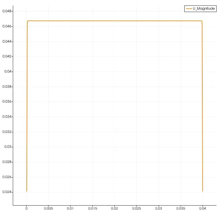
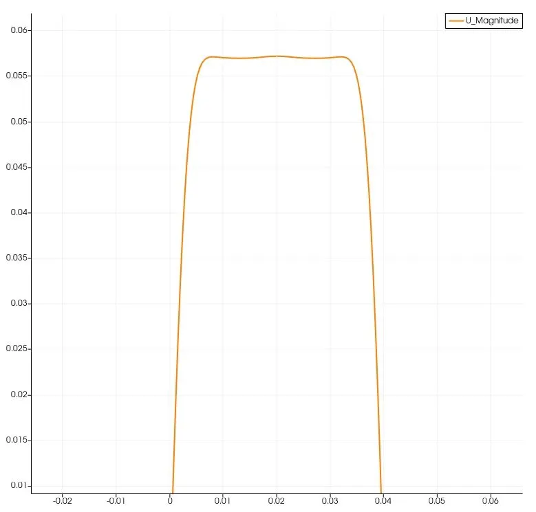
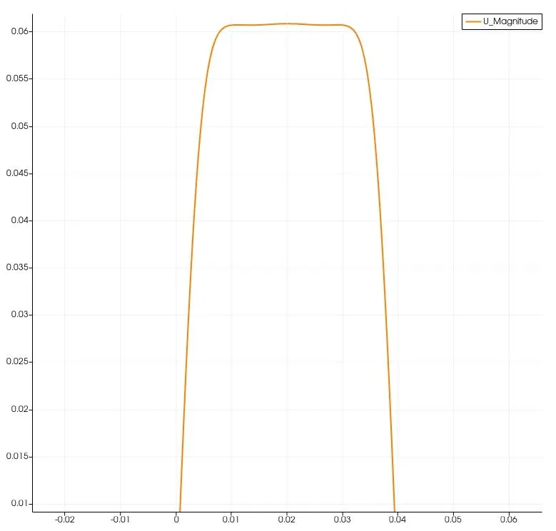
2. Velocity profiles
a. At entrance
b. At x=0.1
c. At x=0.2
d. At x=0.5
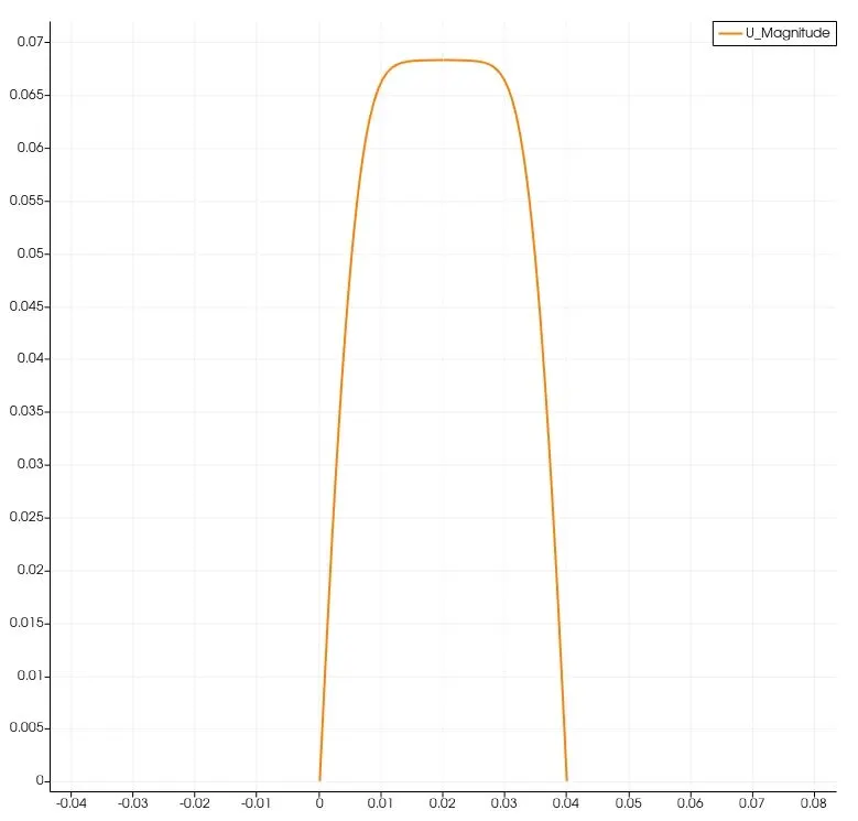
e. At x=1
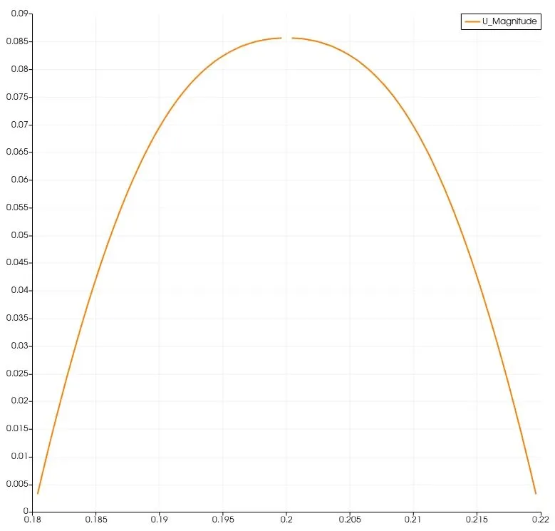
f. At x=2
g. At x=4
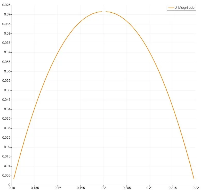
h. At x=5.04
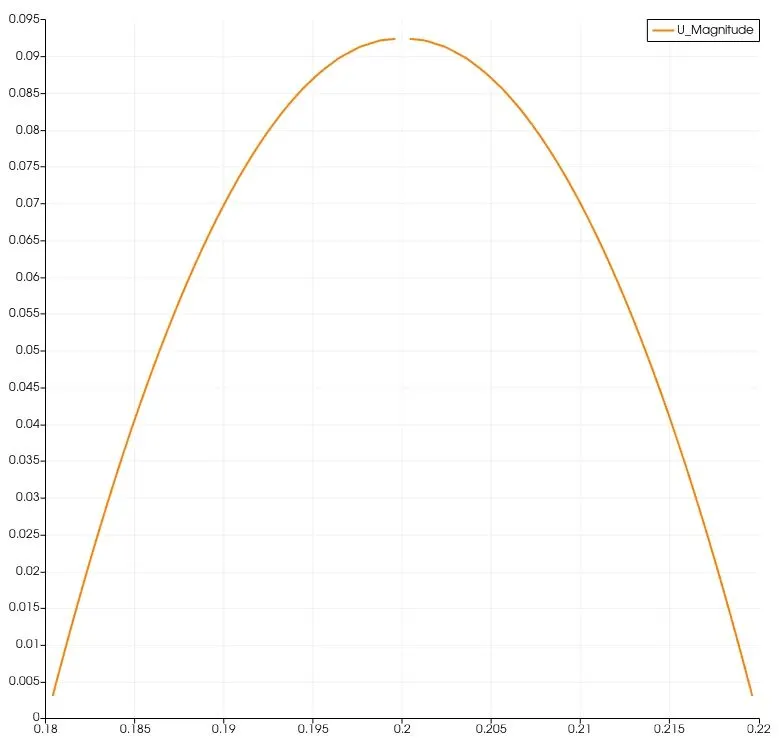
i. At x=6.04
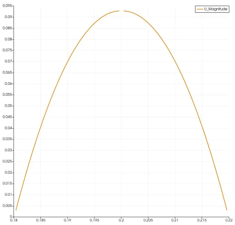
3. Shear Stress Distribution
The following diagram is plotted for only upper half of pipe
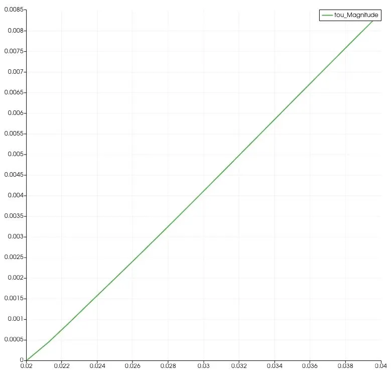
Comment: This plot matches with the plot obtained by analytical mathod for Hagen Poiseuille Flow.
4. Pressure
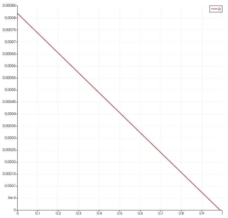
In above diagram, the guage pressure at exit of pipe is 0 atm (Exposed to atmosphere). And Pressure distribution is also correct since flow is exiting from outlet which has low pressure and the same is validated from equation
dp= 64*(v^2)*Lt/(Re*2*D)
dp is directly proportional to length of pipe (Lt). Hence a straight line relationship is expected.
B. For angle 25
radius=4 cm
# BlockMesh file generated by MATLAB
FoamFile
{
	version     2.0;
	format      ascii;
	class       dictionary;
	object      blockMeshDict;
}
//******************************//
scale 1;
vertices
(
	(0 0 0)
	(0 0.039052 0.008658)
	(0 0.039052 -0.008658)
	(11.080000 0 0)
	(11.080000 0.039052 0.008658)
	(11.080000 0.039052 -0.008658)
);
blocks
(
hex (0 3 5 2 0 3 4 1) (100 20 1) simpleGrading (1 0.1 1)
);
edges
(
arc 1 2 (0 0.040000 0)
arc 4 5 (11.080000 0.040000 0)
);
boundary
(
	 inlet
	 {
		 type patch;
		 faces
		 (
			(0 1 2 0)
		 );
	 }
	 outlet
	 {
		 type patch;
		 faces
		 (
			(3 5 4 3)
		 );
	 }
	 front
	 {
		 type symmetry;
		 faces
		 (
			(0 3 4 1)
		 );
	 }
	 back
	 {
		 type symmetry;
		 faces
		 (
			(0 2 5 3)
		 );
	 }
	 axis
	 {
		 type empty;
		 faces
		 (
			(0 3 3 0)
		 );
	 }
	 pipeWall
	 {
		 type wall;
		 faces
		 (
			(1 4 5 2)
		 );
	 }
);
mergePatchPairs
(
);
//******************************//
The formed mesh is:
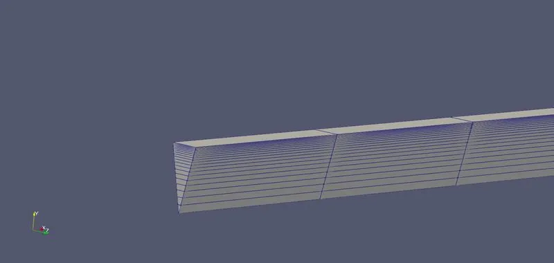
velocity is calculated from Raynold's number
Velocity(v)=0.0234 m/s
Total Simulation time: ntime=Lt/v=470.3223 sec
## Results
1. Entrance Length
Entrance length is calculated as: Le=0.06*Re*2*r
In this case, r=0.02 and Re= 2100
Hence Le= 10.08m
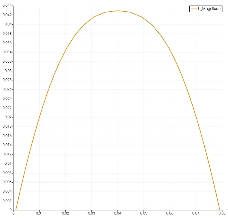
2. Velocity Profiles
a. At entrance
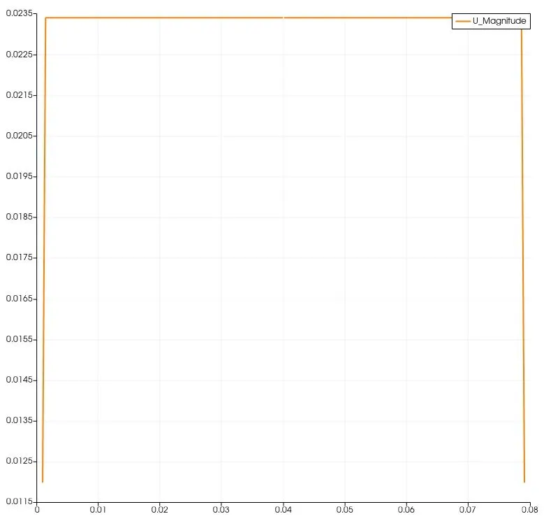
b. At x=0.1m
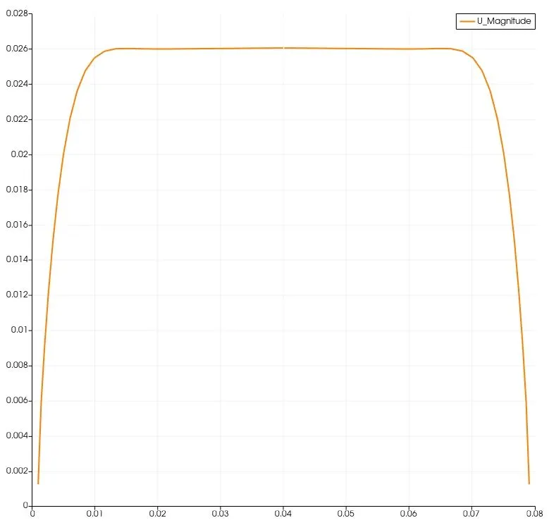
c. At x=0.2m
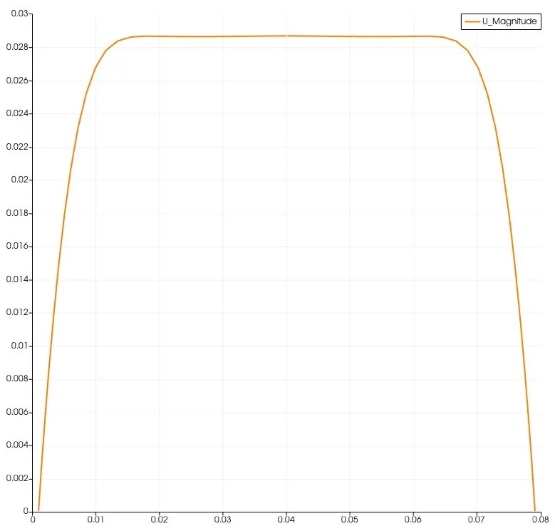
d. At x=0.5m
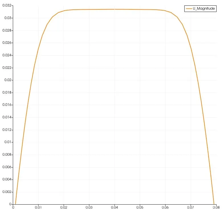
e. At x=1m
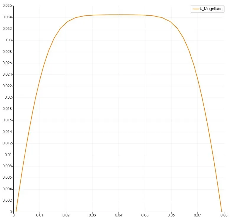
f. At x=2m
g. At x=4m
3. Shear Stress Profile
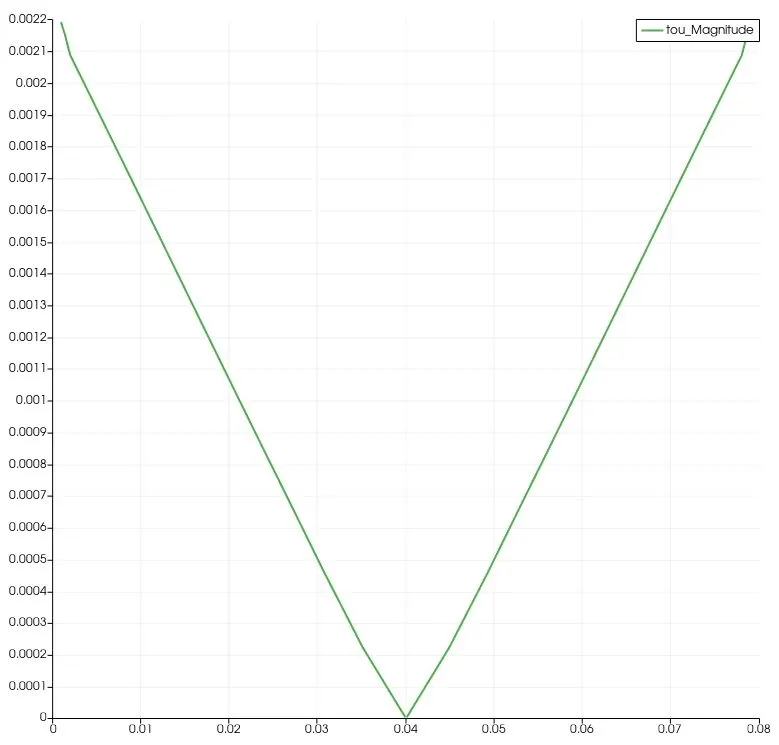
The above plot is plotted for full pipe (y=-0.04m to y=0.04m) By looking at x axis, the total span is 0.08m which is equal to diameter of pipe. The above graph is silimar to graph obtained by analytical method.
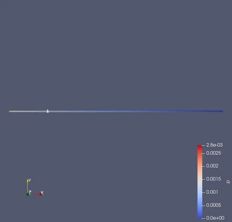
4. Pressure
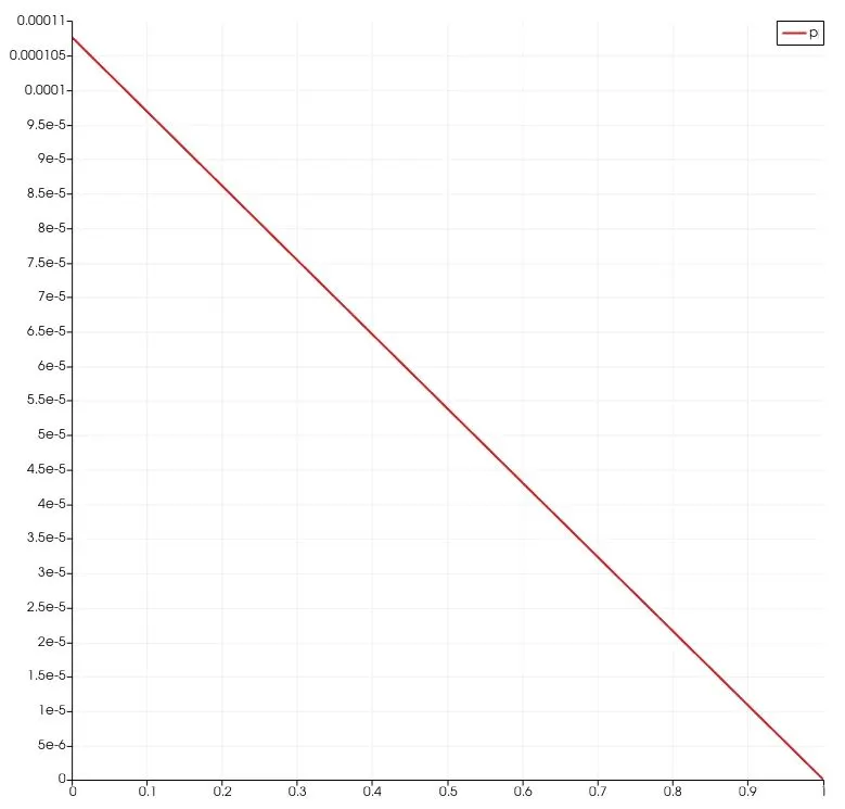
In above diagram, the guage pressure at exit of pipe is 0 atm (Exposed to atmosphere). And Pressure distribution is also correct since flow is exiting from outlet which has low pressure and the same is validated from equation
dp= 64*(v^2)*Lt/(Re*2*D)
dp is directly proportional to length of pipe (Lt). Hence a straight line relationship is expected.
C. For angle 45
radius=0.01m
# Generting blockMesh file fro MATLAB
FoamFile
{
	version     2.0;
	format      ascii;
	class       dictionary;
	object      blockMeshDict;
}
//******************************//
scale 1;
vertices
(
	(0 0 0)
	(0 0.009239 0.003827)
	(0 0.009239 -0.003827)
	(3.520000 0 0)
	(3.520000 0.009239 0.003827)
	(3.520000 0.009239 -0.003827)
);
blocks
(
hex (0 3 5 2 0 3 4 1) (100 20 1) simpleGrading (1 0.1 1)
);
edges
(
arc 1 2 (0 0.010000 0)
arc 4 5 (3.520000 0.010000 0)
);
boundary
(
	 inlet
	 {
		 type patch;
		 faces
		 (
			(0 1 2 0)
		 );
	 }
	 outlet
	 {
		 type patch;
		 faces
		 (
			(3 5 4 3)
		 );
	 }
	 front
	 {
		 type symmetry;
		 faces
		 (
			(0 3 4 1)
		 );
	 }
	 back
	 {
		 type symmetry;
		 faces
		 (
			(0 2 5 3)
		 );
	 }
	 axis
	 {
		 type empty;
		 faces
		 (
			(0 3 3 0)
		 );
	 }
	 pipeWall
	 {
		 type wall;
		 faces
		 (
			(1 4 5 2)
		 );
	 }
);
mergePatchPairs
(
);
//******************************//
The generated mesh is
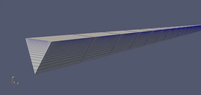
## Results
1. Entrance length:
Entrance length is calculated as: Le=0.06*Re*2*r
In this case, r=0.01 and Re= 2100
Hence Le= 2.52m
2. Velocity Profiles
a. At entrance
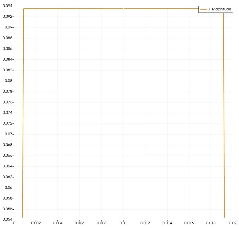
b. At x=0.1m
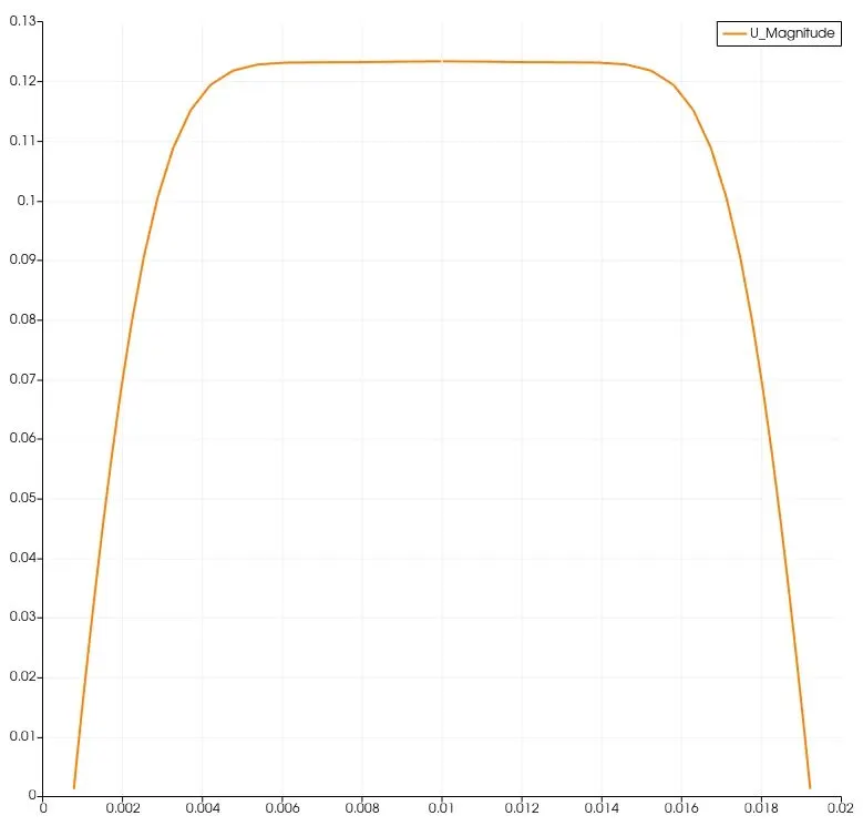
c. At x=0.2m
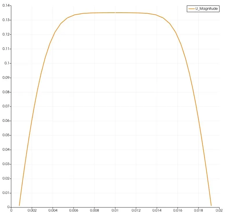
d. At x=0.5m
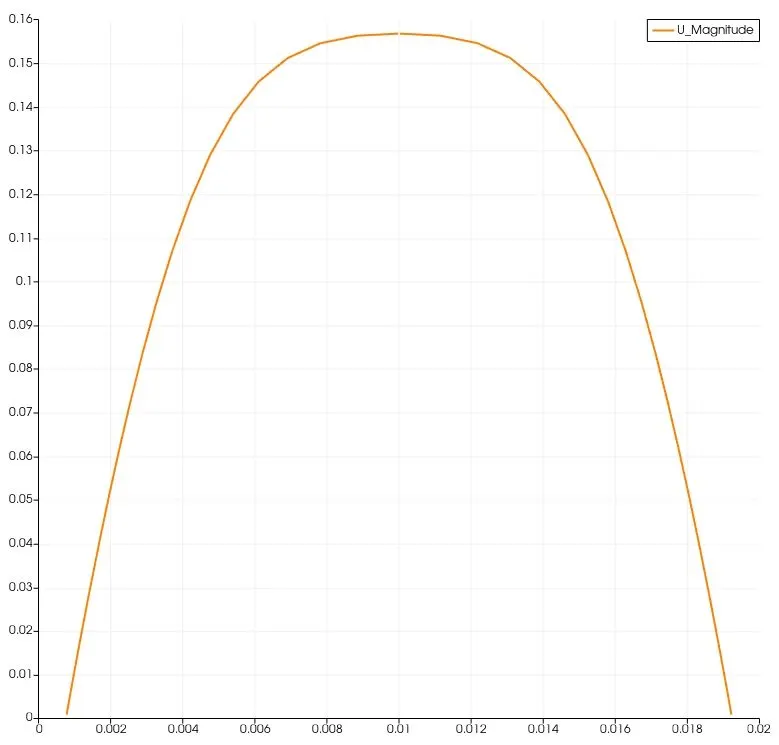
e. At x=1m
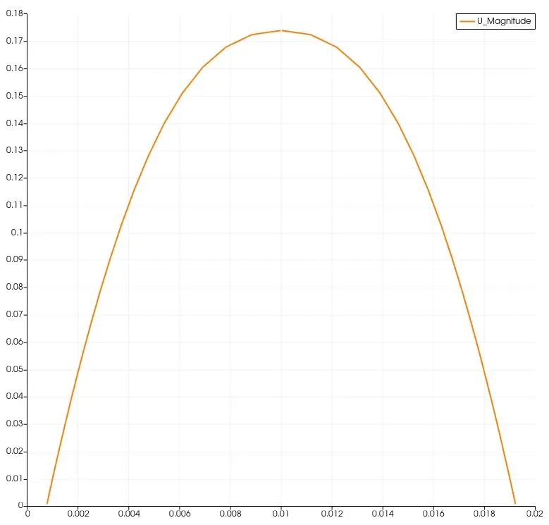
f. At x=2m
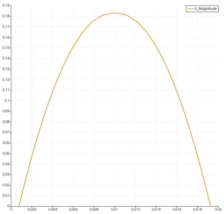
g. At x=2.52m
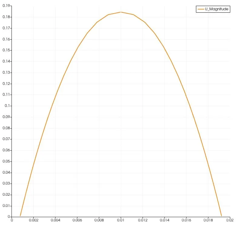
h. At exit
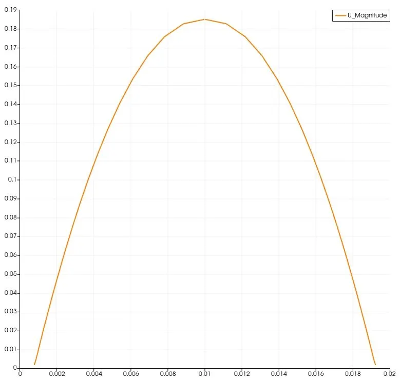
3. Shear Stress Profile
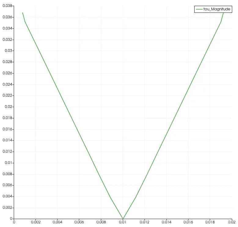
The above diagram is plotted for full diameter of pipe (2cm).
4. Pressure
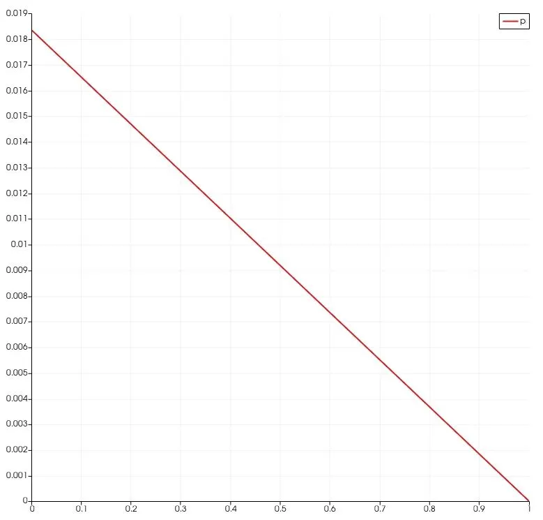
In above diagram, the guage pressure at exit of pipe is 0 atm (Exposed to atmosphere). And Pressure distribution is also correct since flow is exiting from outlet which has low pressure and the same is validated from equation
dp= 64*(v^2)*Lt/(Re*2*D)
dp is directly proportional to length of pipe (Lt). Hence a straight line relationship is expected.