Week 12 - Validation studies of Symmetry BC vs Wedge BC in OpenFOAM vs Analytical H.P equation

WEEK 12 - VALIDATION STUDIES OF SYMMETRY BC VS WEDGE BC IN OpenFOAM VS ANALYTICAL H.P EQUATION

AIM:

• To validate Hydro-dynamic length with the numerical result.
• To validate the fully developed flow velocity profile with its analytical profile.
• Validate maximum velocity and pressured drop for fully developed flow.
• Post-process Shear stress and validate wall shear stress for fully developed flow.
• Highligh the differences in both boundary conditions in terms of their usage and aplication.

ANGLES TO TEST:

• 10 degrees wedge and symmetry
• 25 degrees wedge and symmetry
• 45 degrees wedge and symmetry

PROCEDURE:

STEP-1:

First, we need to install the visual box and then we need to install the ubuntu in our system.

STEP-2:

we need to install the openFOAM software in ubuntu

STEP-3:

Now we need to open the terminal from the ubuntu desktop.

STEP-4:

The terminal is the command window where we can access to the folders, parafoam.

STEP-5:

cd - is the keyword which resembles "current directory"

ls - is the keyword which resembles "list" and it is used to list down the elements inside the folder.

In the terminal, we need to open the tutorials by using the command "cd $FOAM_TUTORIALS"

and followed by is explained in the picture.

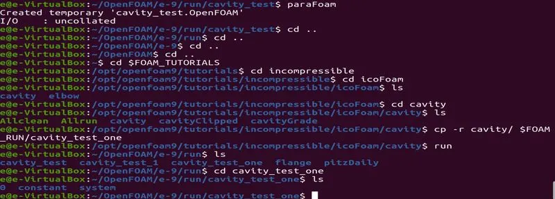
• From the picture we can see that after opening the tutorials we need to choose "cd incompressible", then "cd icoFoam"
• This icoFoam is used to calculate incompressible Navier Stoke's equation.
• From there we need to open the "cd cavity" and we need to copy this file in our directory so that we can run this by using the command "cp -r cavity/$FOAM_RUN/cavity_test".
• This cavity_test is the folder where we are going to save what we require.
• we will be having "0", "constant", "system" after listing down.

STEP-6:

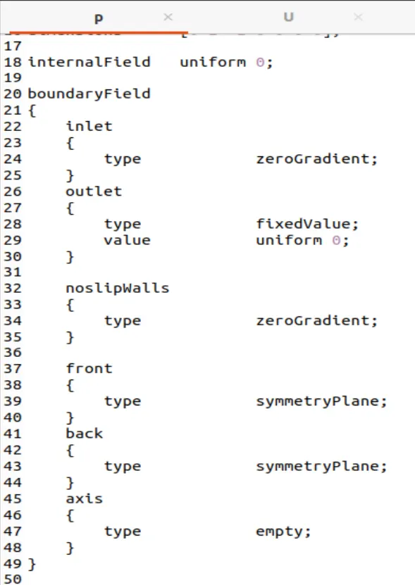
• By selecting "0" we will get two options one is "P" which is pressure and the other is "U", which is velocity. This has to be opened and it as to be edited according to our requirements and this can be done by using the command "gedit p" and "gedit u". "gedit" is a command which is used to open it because it is editable file.
• Now we need to give the values according to our requirements which is shown below.

STEP-7:

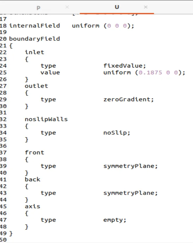
Similarly, we need to do for velocity file.

STEP-8:

• We need to edit the block mesh file or we need to create the file using MATLAB as follows,
• The code for creating symmetry blockmesh file and this also contains analytical solution:

% % % % block mesh file for pipe flow 0f 45 degree symmetry angle
close all
clear
clc

% % initial conditions
% reynold's number
Re = 2100;
% density of water (kg/m^3)
rho = 997;
% dynamic viscosity of water (pa. s)
mu = 8.9 * 10^-4;
% kinematic viscosity of water (m^2/ s)
nu = mu/rho;
% diameter of pipe (m)
D = 0.01;
% radius of pipe (m)
R = D/2;
% area of pipe
A = pi * D^2;
% velocity (m/s)
V = (Re * mu)/(rho * D);
% gravity due to acelleration (m/s^2)
g  = 9.81;
% hydrodynamic length (m)
L_hd = 0.0575 * Re * D;
% total pipe length (m)
L_T = L_hd + 0.2925;
% wedge angle (THETA)
theta = 45;

% % % analytic calculations:
% % velocity calculations:
% average velocity occurs at 0.707 R (ie 3.535e-3 m)
V_avg = V;
% maximum velocity
V_max = 2 * V_avg;
% d = linspace(0,D,1000);
r = linspace(0,R,1000);
% variation of velocity along the radius of pipe
v_d = V_max * (1 - (r.^2/R^2));
L_V = linspace(0,L_T,1000);
% time
T_t = L_T/V_avg;

% discharge
Q = A * V_avg;

% Hagen Poiseuilles's Equation (head loss)
h_L = (32 * mu * V_avg * L_V)/(rho * g * D^2);

% h_L = (p1 - p2)/(rho * g)
% p1 - p2 = dp (pressure drop)
dp = h_L * rho * g;

% power required to overcome a head loss (W-watts)
P = (128 * mu * Q^2 * L_T)/(pi * D^4);

% %shear stress calculations:
% shear stress at boundary (wall shear stress)
ST_B = 8 * mu * V_avg/D;
% variation of shear stress along the radius of pipe
ST_V = (ST_B * r)/R;
% friction factor or Darcy's friction factor or Moody's friction factor
f_f = 64/Re;
% friction co-efficient or Fanning's co-efficient
f_c = f_f/4;

% % Analytical plots
% figure(1)
% plot(r,v_d,'color','g','LineWidth',2)
% title('Velocity distribution along radius')
% xlabel('Radius')
% ylabel('Velocity distribution along radius')
% hold on

% figure(2)
% % plot(L_V,dp,'color','b','LineWidth',2)
% title('pressure distribution along length of pipe')
% xlabel('length of pipe')
% ylabel('pressure')

% figure(3)
% plot(r,ST_V,'color','r','LineWidth',2)
% title('Shear stress distribution along radius')
% xlabel('Radius')
% ylabel('Shear stress distribution along radius')

% figure(4)
% plot(L_V,dp)


% % mesh size
nx = 500;
ny = 50;
nz = 1;

% % to create the file
f1 = fopen('blockMeshDict_45', 'w');

% % file contents
fprintf(f1, 'FoamFile\n');
fprintf(f1, '{\n');
fprintf(f1, '     version      2.0;\n');
fprintf(f1, '     format       ascii;\n');
fprintf(f1, '     class        dictionary;\n');
fprintf(f1, '     object       blockMeshDict;\n');
fprintf(f1, '}\n\n\n');

fprintf(f1, 'convertTometers 1;\n\n');

fprintf(f1, 'vertices\n');
fprintf(f1, '(\n');
fprintf(f1, '     (0 0 0)\n');
%fprintf(f1, '     (0 R * cosd(theta/2) R * sind(theta/2))\n');
fprintf(f1, '     (%f\t   %f\t%f)\n',0, R * cosd(theta/2), R * sind(theta/2));

%fprintf(f1, '     (0 R * cosd(theta/2) -R * sind(theta/2),\n');
fprintf(f1, '     (%f\t   %f\t%f)\n',0, R * cosd(theta/2),-R * sind(theta/2));

%fprintf(f1, '     (L_T 0 0)\n');
fprintf(f1, '     (%f\t   %f\t%f)\n',L_T, 0, 0);

%fprintf(f1, '     (L_T R * cosd(theta/2) R * sind(theta/2))\n');
fprintf(f1, '     (%f\t   %f\t%f)\n',L_T, R * cosd(theta/2), R * sind(theta/2));

%fprintf(f1, '     (L_T R * cosd(theta/2) -R * sind(theta/2))\n');
fprintf(f1, '     (%f\t   %f\t%f)\n',L_T, R * cosd(theta/2),-R * sind(theta/2));
fprintf(f1, ');\n\n');

fprintf(f1, 'blocks\n');
fprintf(f1, '(\n');
%fprintf(f1,'      hex (0 3 5 2 0 3 4 1) (nx ny nz) simpleGrading (1 1 1)\n');
fprintf(f1, '      hex (%d %d %d %d %d %d %d %d) (%d %d %d) simpleGrading (1 1 1)\n',0, 3, 5, 2, 0, 3, 4, 1, nx, ny, nz);
fprintf(f1, ');\n\n');
fprintf(f1, 'edges\n');
fprintf(f1, '(\n');

%fprintf(f1, '      arc 1 2 (0 R 0)\n');
fprintf(f1,'       arc 1 2 (0 %f 0)\n',R);
%fprintf(f1, '      arc 4 5 (L_T R 0)\n');
fprintf(f1,'       arc 4 5 (%d %f 0)\n',L_T,R);
fprintf(f1, ');\n\n');

fprintf(f1, 'boundary\n');
fprintf(f1, '(\n');
fprintf(f1, '      inlet\n');
fprintf(f1, '      {\n');
fprintf(f1, '          type patch;\n');
fprintf(f1, '          faces\n');
fprintf(f1, '          (\n');
fprintf(f1, '              (0 1 2 0)\n');
fprintf(f1, '          );\n');
fprintf(f1, '      }\n');

fprintf(f1, '      outlet\n');
fprintf(f1, '      {\n');
fprintf(f1, '          type patch;\n');
fprintf(f1, '          faces\n');
fprintf(f1, '          (\n');
fprintf(f1, '              (3 5 4 3)\n');
fprintf(f1, '          );\n');

fprintf(f1, '      }\n');

fprintf(f1, '      front\n');
fprintf(f1, '      {\n');
fprintf(f1, '          type symmetryPlane\n');
fprintf(f1, '          faces\n');
fprintf(f1, '          (\n');
fprintf(f1, '              (0 3 4 1)\n');
fprintf(f1, '          );\n');
fprintf(f1, '      }\n');

fprintf(f1, '      back\n');
fprintf(f1, '      {\n');
fprintf(f1, '          type symmetryPlane;\n');
fprintf(f1, '          faces\n');
fprintf(f1, '          (\n');
fprintf(f1, '              (0 2 5 3)\n');
fprintf(f1, '          );\n');
fprintf(f1, '      }\n');


fprintf(f1, '      noslipWalls\n');
fprintf(f1, '      {\n');
fprintf(f1, '          type wall;\n');
fprintf(f1, '          faces\n');
fprintf(f1, '          (\n');
fprintf(f1, '              (2 1 4 5)\n');
fprintf(f1, '          );\n');
fprintf(f1, '      }\n');

fprintf(f1, '      axis\n');
fprintf(f1, '      {\n');
fprintf(f1, '          type empty;\n');
fprintf(f1, '          faces\n');
fprintf(f1, '          (\n');
fprintf(f1, '              (0 3 3 0)\n');
fprintf(f1, '          );\n');
fprintf(f1, '      }\n');

fprintf(f1, ');\n\n');

fprintf(f1, 'mergePatchPairs\n');
fprintf(f1, '(\n');
fprintf(f1, ');');

STEP-9:

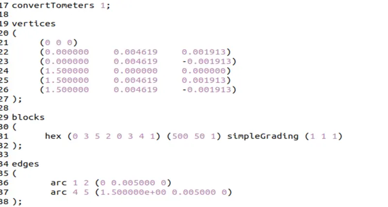
• Now we need to open "system" and there we need to select "blockMeshDict" and we need to replace file which has been created using MATLAB:
• "hex" is the keyword which resembles the type of mesh.
• Next to that is numbered faces of five geometry blocks.
• Next to that is to define number of cells along x, y and z axis.
• "simpleGrading" is the keyword which resembles grading factor and here in this case - 1 is "1".
• This part is to generate mesh.
• if there is wedge type problems, then we need to define edges also.

STEP-10:

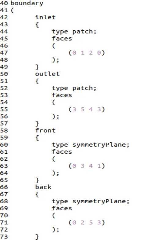
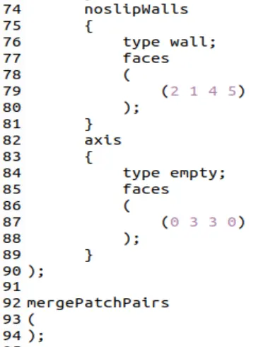
• In the blockMeshDict itself, we need to give the following details.
• We need to give boundary conditions such as "inlet", "outlet", "frontandback", "axis" and "noslipwalls"

STEP-11:

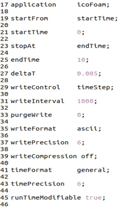
• Now we need to open "system" and there we need to select "controlDict" and we need to edit the following:
• We need to make sure that CFL number should be less than "0.5"

STEP-12:

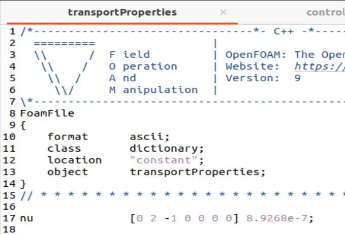
Now, we need to change the value of kinematic viscosity value in the "transportProperties"

STEP-13:

After completing all these settings, we need to save the things what we have done by pressing the "save" button which is on the right side top or "ctrl + s"

STEP-14:

Now we need to go back to the terminal and we need to give the command "blockMesh"

STEP-15:

Now the mesh generation is done. Then we need to solve the problem by using "icoFoam" solver.

STEP-16:

To view the simulation or simulated results, we need to open paraview and to that we need to give the command "paraFoam"

RESULTS AND OUTPUT:

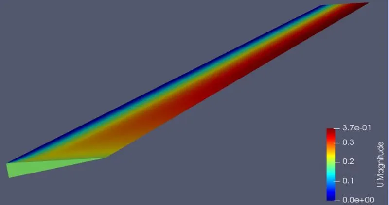
velocity plot of wedge 10 deg:

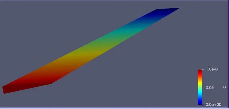
pressure plot of 10 deg:

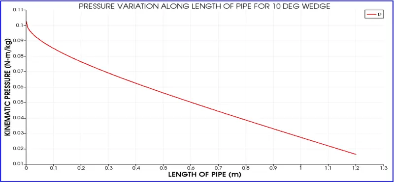
pressure variation upto hydrodynamic length

pressure variation from hydrdynamic length to total length

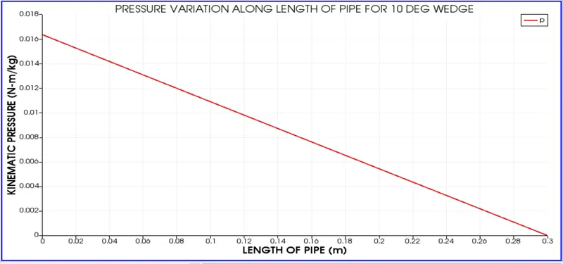
From the above graphs, we can observe that till hydrodynamic length pressure varies little parabolically and from hydrodynamic length it varies linearly.

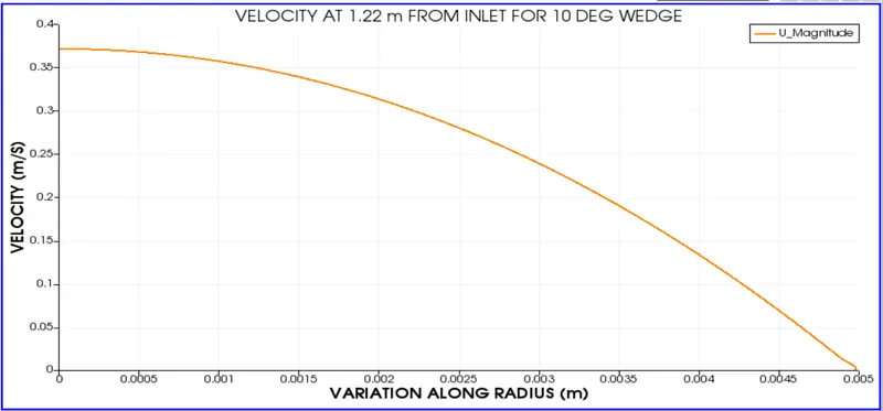
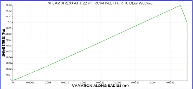
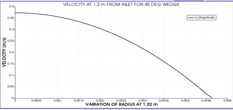
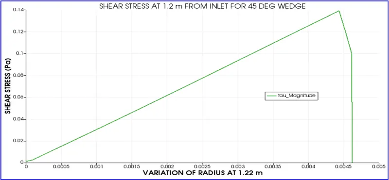
velocity and shear stress plots for 10, 25, 45 degree wedge:

1. 10 DEGREE

2. 25 DEGREE:

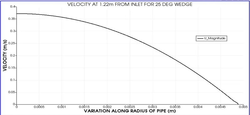
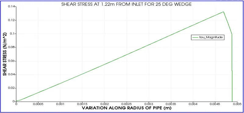
3. 45 DEGREE:

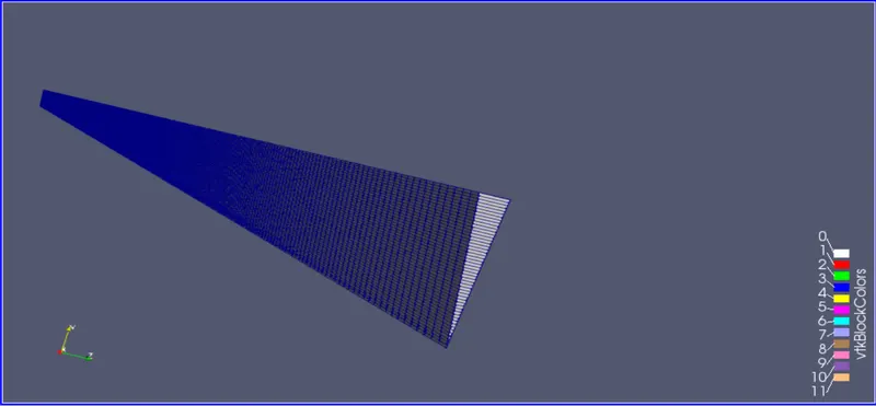
Meshed structure of 10 degree symmetry:

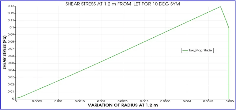
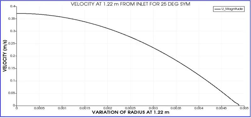
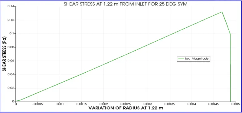
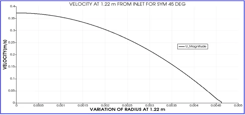
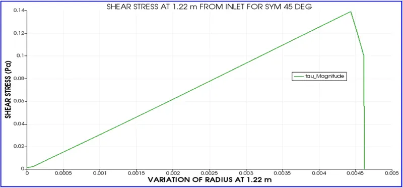
velocity and shear stress plots for 10, 25, 45 degree symmetry:

1. 10 DEGREE

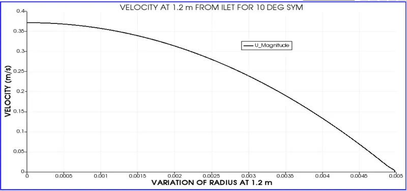
2. 25 DEGREE

3. 45 degree:

Difference between wedge and symmetry:

Wedge boundary condition:

The openFOAM solves the solution by converting cartesian co-ordinates to polar co-ordinates.

symmetry boundary condition:

The openFOAM solves the solution in cartesian co-ordinates without any conversion.

CONCLUSION:

• By seeing the plots it is impossible to conclude the approximations, so we need to take the values in spread sheet and we need to do the approximations comparing with the analytic values.
• By doing that, I came to a conclusion when the wedge angle increases accuracy to analytic solution is decreased and comparing 4 degree wedge with analytic, the results are very close to eachother, but comparing 10, 25, 45 degree wedges, I felt there is no much difference between them by evaluating and comparing 4 degree with 10, 25 and 45 degree wedges, where, considerable difference was observed.
• For the approximations I have calculated at the point 1.22 m from inlet and at radius 0.00459
• Shear stress approximations: for 10 degrees, the error percentage was 1. 25%, for 25 degrees 5% and for 45 degrees it was more than 10 percent.
• velocity approximations : for 10 degrees, the error percentage was 3.18%, for 25 degrees 26% and for 45 degrees it was more than 80 percent.
• By comparing wedge and symmetry, I found there is no much difference in the values point of view.
• The most important thing is as wedge angle increases, in paraFoam radius gets decreased so the results gets deviated.
• From this we can say that wedge angle must be less than 5 degree, so that results will be close to analytic solution and also computational time is less compared to higher degree wedge.