Week 11 - Simulation of Flow through a pipe in OpenFoam
In nonideal fluid dynamics, the Hagen–Poiseuille equation, also known as the Hagen–Poiseuille law, is a physical law that gives the pressure drop in an incompressible and Newtonian fluid in laminar flow flowing through a long cylindrical pipe of constant cross section. This is applicable after the hydrodynamic entry length
EQUATION:
In standard fluid-kinetics notation.
`DeltaP=frac(32muU_(avg)L)(D^2)`
where:
- ΔP is the pressure difference between the two ends,
- L is the length of pipe,
- μ is the dynamic viscosity,
- Q is the volumetric flow rate,
- R is the pipe radius,
- A is the cross section of pipe.
The equation does not hold close to the pipe entrance.
Given parameters.
- Wedge angle less than 5 degrees,
- Flow is axi symetrical.
- Fluid is incompressible and the flow is laminar.
Expected Velocity Profile.
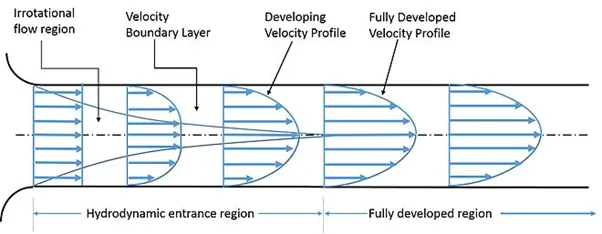
Assuming the following:
- The distance the fluid has to travel to become fully developed is given by the Entry Length formula.
- Given Reynolds number is 2100. This implies flow is laminar.
- Hence Entry length formula for Laminar is given by:`L/D=0.06Re`
- where L is effective length; d is dia of pipe and Re is reyonolds number.
- Assuming the dia of pipe as 10mm; substituting the values, we get L = 1.26 m;
Steps to follow
- First, the geometry is created in the blockmesh Dict file, this is done by creating the file through the matlab code.
- The mesh is generated according to requirement.
- The velocity and preassure bc are applied
- The controlDict file is edited for Simulation run time and timestep;
- After the geometry is input, the simulation can be started by calling 'icoFoam' command in the terminal.
- 'paraFoam' command helps to open paraView
- The shear stress diagram is obtained by post-processing the velocity results obtained from Openfoam.
Matlab programm for automatically generate blockmeshDict file for a wedge angle provided by user
close all; clear all;clc;

%% define diameter,angle and length of the pipe
D=0.01;  r=D/2;  theta=3;    L=2;
%% file parsing
f1 = fopen('blockMeshDict','w');


fprintf(f1,'%s \n','/*--------------------------------*- C++ -*----------------------------------*\');
fprintf(f1,'%s \n',' =========                 |');
fprintf(f1,'%s \n','  \\      /  F ield         | OpenFOAM: The Open Source CFD Toolbox');
fprintf(f1,'%s \n','   \\    /   O peration     | Website:  https://openfoam.org');
fprintf(f1,'%s \n','    \\  /    A nd           | Version:  10');
fprintf(f1,'%s \n','     \\/     M anipulation  |');
fprintf(f1,'%s \n','\*---------------------------------------------------------------------------*/');


fprintf(f1,'%s \n','FoamFile');
fprintf(f1,'%s \n','{');
fprintf(f1,'\t %s \n','format      ascii;');
fprintf(f1,'\t %s \n','class       dictionary;');
fprintf(f1,'\t %s \n','object      blockMeshDict;');
fprintf(f1,'%s \n','}');
fprintf(f1,'// * * * * * * * * * * * * * * * * * * * * * * * * * * * * * * * * * * * * * //\n');
fprintf(f1,'convertToMeters %d;\n',1);

fprintf(f1,'%s \n','vertices');
fprintf(f1,'%s \n','(');

fprintf(f1, '\t(%d %d %d)\n',0,0,0);
fprintf(f1, '\t(%d %f %f)\n',0,r*cosd(theta/2),r*sind(theta/2));
fprintf(f1, '\t(%d %f %f)\n',0,r*cosd(-theta/2),r*sind(-theta/2));
fprintf(f1, '\t(%d %d %d)\n',L,0,0);
fprintf(f1, '\t(%d %f %f)\n',L,r*cosd(theta/2),r*sind(theta/2));
fprintf(f1, '\t(%d %f %f)\n',L,r*cosd(-theta/2),r*sind(-theta/2));
fprintf(f1,'%s \n',');');


fprintf(f1,'%s \n','blocks');
fprintf(f1,'%s \n','(');
fprintf(f1, '\t hex (%d %d %d %d %d %d %d %d)(%d %d %d)',0,3,5,2,0,3,4,1,500,40,1);
fprintf(f1,' simpleGrading (%d %f %d)\n',1,0.2,1);
fprintf(f1,'%s \n',');');

fprintf(f1,'%s \n','edges');
fprintf(f1,'%s \n','(');
fprintf(f1, '\t arc %d %d (%d %f %d)\n',1,2,0,r,0);
fprintf(f1, '\t arc %d %d (%d %f %d)\n',4,5,L,r,0);
fprintf(f1,'%s \n',');');


fprintf(f1,'%s \n','boundary');
fprintf(f1,'%s \n','(');

fprintf(f1,'\t %s \n','inlet');
fprintf(f1,'\t %s \n','{');
fprintf(f1,'\t \t %s \n','type patch;');
fprintf(f1,'\t \t %s \n','faces');
fprintf(f1,'\t \t %s \n','(');
fprintf(f1, '\t \t \t (%d %d %d %d)\n',0,1,2,0);
fprintf(f1,'\t \t %s \n',');');
fprintf(f1,'\t %s \n','}');

fprintf(f1,'\t %s \n','outlet');
fprintf(f1,'\t %s \n','{');
fprintf(f1,'\t \t %s \n','type patch;');
fprintf(f1,'\t \t %s \n','faces');
fprintf(f1,'\t \t %s \n','(');
fprintf(f1, '\t \t \t (%d %d %d %d)\n',3,4,5,3);
fprintf(f1,'\t \t %s \n',');');
fprintf(f1,'\t %s \n','}');

fprintf(f1,'\t %s \n','Axis');
fprintf(f1,'\t %s \n','{');
fprintf(f1,'\t \t %s \n','type empty;');
fprintf(f1,'\t \t %s \n','faces');
fprintf(f1,'\t \t %s \n','(');
fprintf(f1, '\t \t \t (%d %d %d %d)\n',0,3,3,0);
fprintf(f1,'\t \t %s \n',');');
fprintf(f1,'\t %s \n','}');

fprintf(f1,'\t %s \n','fixedWalls');
fprintf(f1,'\t %s \n','{');
fprintf(f1,'\t \t %s \n','type wall;');
fprintf(f1,'\t \t %s \n','faces');
fprintf(f1,'\t \t %s \n','(');
fprintf(f1, '\t \t \t (%d %d %d %d)\n',1,4,5,2);
fprintf(f1,'\t \t %s \n',');');
fprintf(f1,'\t %s \n','}');

fprintf(f1,'\t %s \n','Wedge');
fprintf(f1,'\t %s \n','{');
fprintf(f1,'\t \t %s \n','type symmetry;');
fprintf(f1,'\t \t %s \n','faces');
fprintf(f1,'\t \t %s \n','(');
fprintf(f1, '\t \t \t (%d %d %d %d)\n',0,3,5,2);
fprintf(f1, '\t \t \t (%d %d %d %d)\n',0,3,4,1);
fprintf(f1,'\t \t %s \n',');');
fprintf(f1,'\t %s \n','}');


fprintf(f1,'%s \n',');');


fprintf(f1,'%s \n','mergePatchPairs');
fprintf(f1,'%s \n','(');
fprintf(f1,'%s \n',');');
fprintf(f1,'%s','// ************************************************************************* //');
fclose(f1);

%% Analytical calculation
v_avg=0.21;
R=r; mu=0.0010016;
r_array=linspace(0,R,40);
v=2*v_avg*(1-(r_array.^2)/R^2);

figure(1)
plot(r_array,v);
xlabel('Pipe Radius(R)');
ylabel('Velocity profile');
title('Velocity profile for a fully developed flow along pipe radius');

for i=1:39
    tau(i+1)=mu*( (v(i+1)-v(i)) / (r_array(i+1)-r_array(i)) );
end
    figure(2)
    plot(r_array,tau);
    xlabel('Pipe Radius(R)');
    ylabel('Shear Stress profile');
    title('Shear Stress profile for a fully developed flow along pipe radius');

L_h=1.26;
L_fd=L-L_h;
deltaP=32*mu*v_avg*L_fd/(D^2);
L_fdarray=linspace(0,L_fd,200);
deltaP_array=linspace(deltaP,0,200);


figure(3)
plot(L_fdarray,deltaP_array);
xlabel('Length of the pipe(X axis)');
ylabel('Pressure');
title('Pressure drop for a fully developed flow along the length of the pipe');
BlockMesh Dict file
/*--------------------------------*- C++ -*----------------------------------*\
 =========                 |
  \\      /  F ield         | OpenFOAM: The Open Source CFD Toolbox
   \\    /   O peration     | Website:  https://openfoam.org
    \\  /    A nd           | Version:  10
     \\/     M anipulation  |
\*---------------------------------------------------------------------------*/

FoamFile
{
	 format      ascii;
	 class       dictionary;
	 object      blockMeshDict;
}
// * * * * * * * * * * * * * * * * * * * * * * * * * * * * * * * * * * * * * //
convertToMeters 1;

vertices
(
	(0 0 0)
	(0 4.998287e-03 1.308847e-04)
	(0 4.998287e-03 -1.308847e-04)
	(2 0 0)
	(2 4.998287e-03 1.308847e-04)
	(2 4.998287e-03 -1.308847e-04)
);
blocks
(
	 hex (0 3 5 2 0 3 4 1)(500 40 1) simpleGrading (1 0.2 1)
);
edges
(
	arc 1 2 (0 0.005 0)
	arc 4 5 (2 0.005 0)
);
boundary
(
	 inlet
	 {
	 	 type patch;
	 	 faces
	 	 (
	 	 	 (0 1 2 0)
	 	 );
	 }
	 outlet
	 {
	 	 type patch;
	 	 faces
	 	 (
	 	 	 (3 4 5 3)
	 	 );
	 }
	 Axis
	 {
	 	 type empty;
	 	 faces
	 	 (
	 	 	 (0 3 3 0)
	 	 );
	 }
	 fixedWalls
	 {
	 	 type wall;
	 	 faces
	 	 (
	 	 	 (1 4 5 2)
	 	 );
	 }
	 Wedge
	 {
	 	 type symmetry;
	 	 faces
	 	 (
	 	 	 (0 3 5 2)
	 	 	 (0 3 4 1)
	 	 );
	 }
);
mergePatchPairs
(
);

// ************************************************************************* //
VELOCITY BOUNDARY CONDITIONS
/*--------------------------------*- C++ -*----------------------------------*\
  =========                 |
  \\      /  F ield         | OpenFOAM: The Open Source CFD Toolbox
   \\    /   O peration     | Website:  https://openfoam.org
    \\  /    A nd           | Version:  10
     \\/     M anipulation  |
\*---------------------------------------------------------------------------*/
FoamFile
{
    format      ascii;
    class       volVectorField;
    object      U;
}
// * * * * * * * * * * * * * * * * * * * * * * * * * * * * * * * * * * * * * //

dimensions      [0 1 -1 0 0 0 0];

internalField   uniform (0 0 0);

boundaryField
{
    inlet
    {
        type            fixedValue;
        value           uniform (0.21 0 0);
    }
    outlet
    {
        type            zeroGradient;
    }
    Axis
    {
	 type            empty;
    }

    fixedWalls
    {
        type            noSlip;
    }

    Wedge
    {
        type            symmetry;
    }

}

// ************************************************************************* //
The velocity in x direction is calculated such that the Reynold's number is 2100.
`Re=frac(rhov_(avg)D)(mu)`
Kinematic viscosity = `nu=mu/rho`
`Re=frac(v_(avg)D)(nu)`
Use the following data for water at 20*C
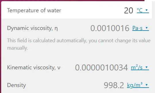
Substitute it in the equation of `Re=frac(v_(avg)D)(nu)` and find the velocity v.
Re=2100;
The velocity `v=0.21 m/s`;
PRESSURE BOUNDARY CONDITIONS
/*--------------------------------*- C++ -*----------------------------------*\
  =========                 |
  \\      /  F ield         | OpenFOAM: The Open Source CFD Toolbox
   \\    /   O peration     | Website:  https://openfoam.org
    \\  /    A nd           | Version:  10
     \\/     M anipulation  |
\*---------------------------------------------------------------------------*/
FoamFile
{
    format      ascii;
    class       volScalarField;
    object      p;
}
// * * * * * * * * * * * * * * * * * * * * * * * * * * * * * * * * * * * * * //

dimensions      [0 2 -2 0 0 0 0];

internalField   uniform 0;

boundaryField
{
    inlet
    {
        type            zeroGradient;
    }
   outlet
    {
        type            fixedValue;
	  value		uniform 0;
    }
    Axis
    {
        type            empty;
    }

    fixedWalls
    {
        type            zeroGradient;
    }
    Wedge
    {
        type            symmetry;
    }

}

// ************************************************************************* //
Physical Properties
/*--------------------------------*- C++ -*----------------------------------*\
  =========                 |
  \\      /  F ield         | OpenFOAM: The Open Source CFD Toolbox
   \\    /   O peration     | Website:  https://openfoam.org
    \\  /    A nd           | Version:  10
     \\/     M anipulation  |
\*---------------------------------------------------------------------------*/
FoamFile
{
    format      ascii;
    class       dictionary;
    location    "constant";
    object      physicalProperties;
}
// * * * * * * * * * * * * * * * * * * * * * * * * * * * * * * * * * * * * * //

nu              [0 2 -1 0 0 0 0] 1e-6;


// ************************************************************************* //
The value of `nu` is set to 1e-6 such that the value is at 20*C
ControlDict
/*--------------------------------*- C++ -*----------------------------------*\
  =========                 |
  \\      /  F ield         | OpenFOAM: The Open Source CFD Toolbox
   \\    /   O peration     | Website:  https://openfoam.org
    \\  /    A nd           | Version:  10
     \\/     M anipulation  |
\*---------------------------------------------------------------------------*/
FoamFile
{
    format      ascii;
    class       dictionary;
    location    "system";
    object      controlDict;
}
// * * * * * * * * * * * * * * * * * * * * * * * * * * * * * * * * * * * * * //

application     icoFoam;

startFrom       startTime;

startTime       0;

stopAt          endTime;

endTime         10;

deltaT          0.002;

writeControl    timeStep;

writeInterval   20;

purgeWrite      0;

writeFormat     ascii;

writePrecision  6;

writeCompression off;

timeFormat      general;

timePrecision   6;

runTimeModifiable true;


// ************************************************************************* //
The simulation is needed to be run for 10 sec because it takes 10 sec for the fluid to travel from inlet to outlet. After 10 sec only, the flow is steady state.
The timestep deltaT=0.002, such that the Courant number is less than 0.5.
fvSchemes
/*--------------------------------*- C++ -*----------------------------------*\
  =========                 |
  \\      /  F ield         | OpenFOAM: The Open Source CFD Toolbox
   \\    /   O peration     | Website:  https://openfoam.org
    \\  /    A nd           | Version:  10
     \\/     M anipulation  |
\*---------------------------------------------------------------------------*/
FoamFile
{
    format      ascii;
    class       dictionary;
    location    "system";
    object      fvSchemes;
}
// * * * * * * * * * * * * * * * * * * * * * * * * * * * * * * * * * * * * * //

ddtSchemes
{
    default         Euler;
}

gradSchemes
{
    default         Gauss linear;
    grad(p)         Gauss linear;
}

divSchemes
{
    default         none;
    div(phi,U)      Gauss linear;
}

laplacianSchemes
{
    default         Gauss linear orthogonal;
}

interpolationSchemes
{
    default         linear;
}

snGradSchemes
{
    default         orthogonal;
}


// ************************************************************************* //
fvSolution
/*--------------------------------*- C++ -*----------------------------------*\
  =========                 |
  \\      /  F ield         | OpenFOAM: The Open Source CFD Toolbox
   \\    /   O peration     | Website:  https://openfoam.org
    \\  /    A nd           | Version:  10
     \\/     M anipulation  |
\*---------------------------------------------------------------------------*/
FoamFile
{
    format      ascii;
    class       dictionary;
    location    "system";
    object      fvSolution;
}
// * * * * * * * * * * * * * * * * * * * * * * * * * * * * * * * * * * * * * //

solvers
{
    p
    {
        solver          PCG;
        preconditioner  DIC;
        tolerance       1e-06;
        relTol          0.05;
    }

    pFinal
    {
        $p;
        relTol          0;
    }

    U
    {
        solver          smoothSolver;
        smoother        symGaussSeidel;
        tolerance       1e-05;
        relTol          0;
    }
}

PISO
{
    nCorrectors     2;
    nNonOrthogonalCorrectors 0;
    pRefCell        0;
    pRefValue       0;
}


// ************************************************************************* //
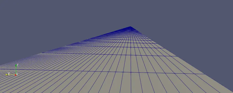
Meshed Geometry:
The isometric view of the mesh is shown. Mesh grading is given only for the walls.
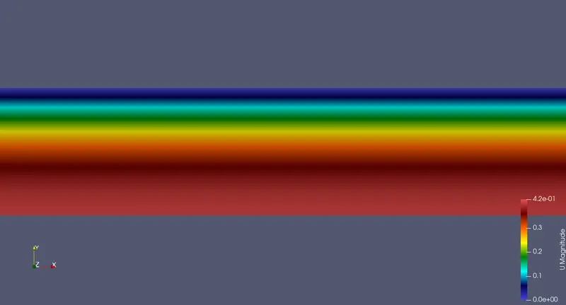
Velocity contour after simulation
OUTPUT PLOT
a) Velocity along the centre line of pipe
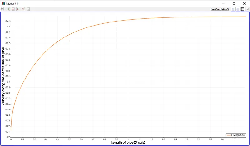
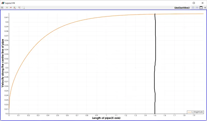
From the graph, it is observed that the velocity profile remains constant after some certain length. It is called hydrodynamic entry length. From graph, it is observed that nearly at 1.5 m from the inlet, the velocity remains constant.
From analytical value it is found that the hydrodynamic length = 1.26 m. So, the hydrodynamic entry length is closely matching with analytical result.
`L/D=0.06Re`
Re=2100; D = 10 mm = 0.01 m;
L = 1.26 m;
b) Velocity along the radius of pipe at different distance from inlet
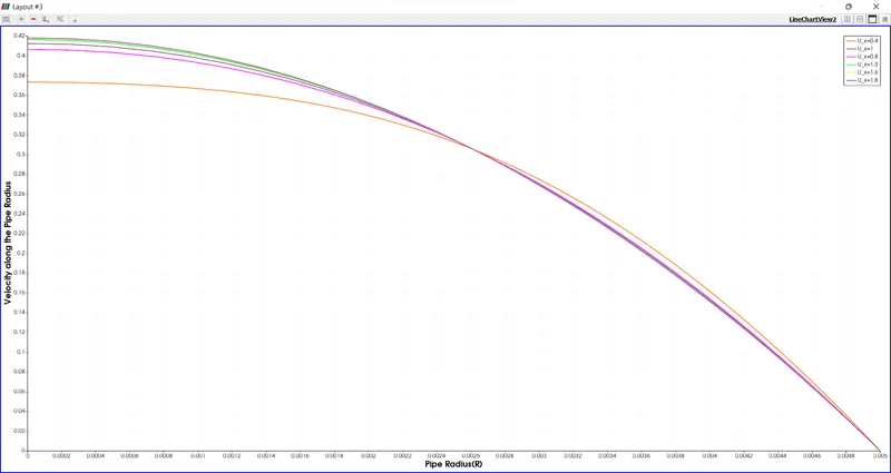
It is found that after 1.3 m from inlet, the graph of velocity at x=1.3, x=1.6 and x=1.8 overlap each other. This validates the hydrodynamic entry length. It shows that if the flow is fully developed, the velocity profile is constant.
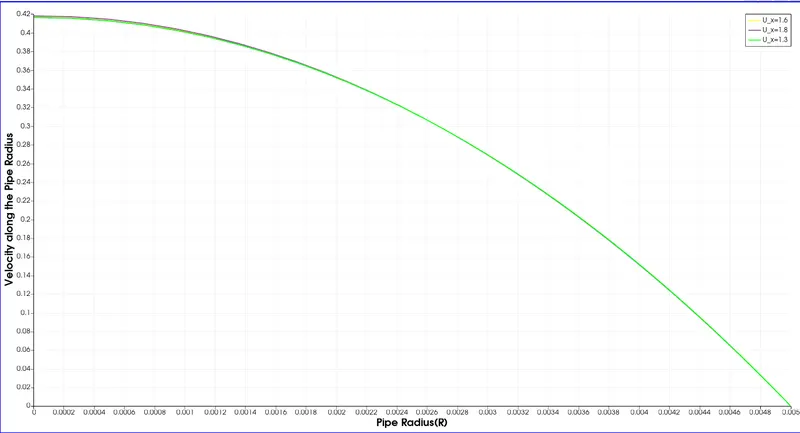
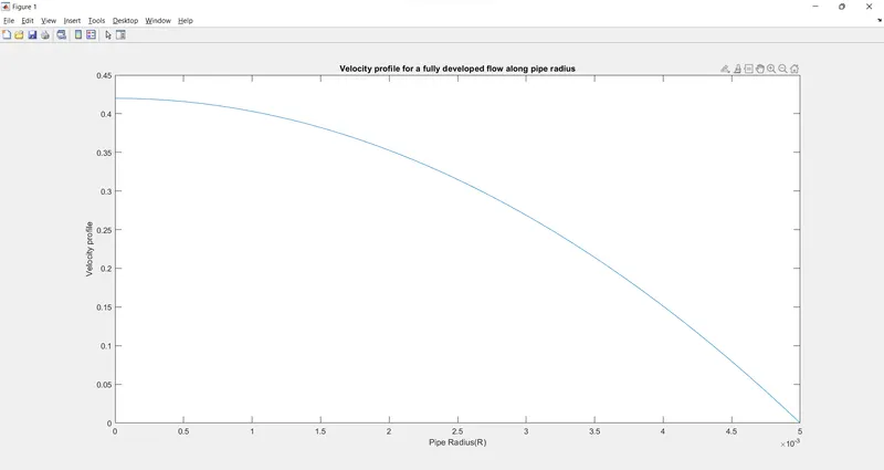
The above figure shows the velocity profile vs pipe radius analytically.
We observed that the analytical result and simulation result have same velocity profile after fully developed zone. This validates the simulation.
c) Shear stress in pipe flow
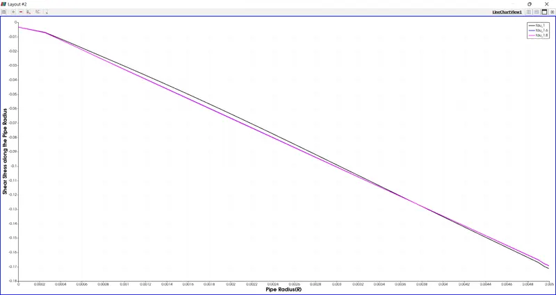
The maximum wall shear stress is given by the formula
`tau_(wall) = -(4muv_(avg))/R`
`T=20 ^0C;`
`mu=0.0010016; v_(avg)=0.21; R=0.005;`
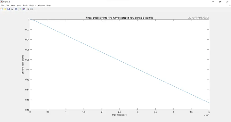
`tau_(wall)=0.168 Pa`
From the graph also, we get the same result for maximum shear stress from simulation also.
The analytical profile is shown below
d) Pressure drop along the length of pipe
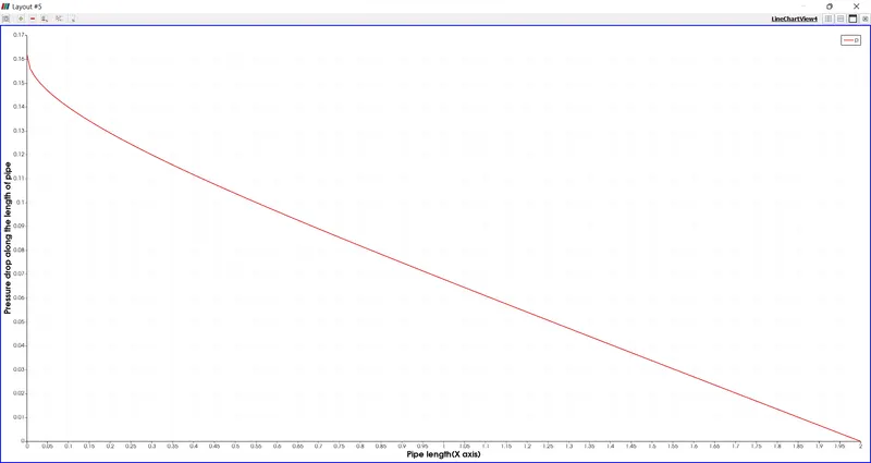
The figure shows that after the hydrodynamic entry region, the pressure drop is constant. this means the slope of the curve is constant and the curve is linear. This means `(dP)/(dx)=constant`
The pressure drop between hydrodynamic entry length and outlet is shown below
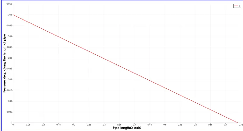
Here, the pressure is kinematic pressure, which is `P/rho`
`rho`=998.2 kg/m3
`P`=49.91 Pa;
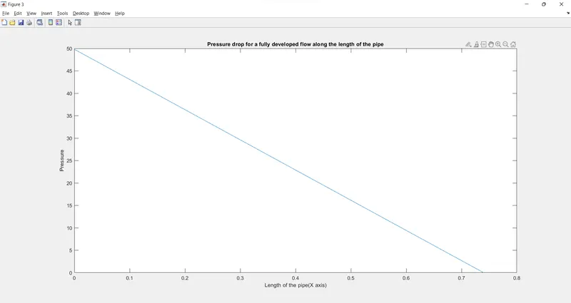
From analytical solution, we get P=49.8076 Pa;
So, the analytical value and simulation result are matching.
Figure shows the analytical value of Pressure drop after hydrodynamic entry length
From analytical solution, `v_(max) = 2v_(avg);`
`v_(max)`=0.42 m/sec;
From graph it is observed that, when the flow is fully developed `v_(max)`=0.418 m/sec;
So, the analytical and simulation results are matching