Week 11 - Simulation of Flow through a pipe in OpenFoam
AIM
To simulate an axi-symmetric flow by applying the wedge boundary condition
Also write code in Matlab to automate the generation of blockMeshDict file. The code should take inputs like pipe length, diameter, wedge angle, etc and output a fully functional blockMeshDict file.
INPUTS
The flow is laminar and flows through a constant cross-section pipe at an inlet Reynold's number of 2100.
Wedge angle should be less than 5 degree
THEORY
The flow through a pipe is the case of internal flow. The surface is the duct in the case of air, it is a pipe in the case of water. The flow is driven because of the pressure difference created by the pumps, air handling units, fans, etc. They find their major application refrigeration and air conditioning industries.
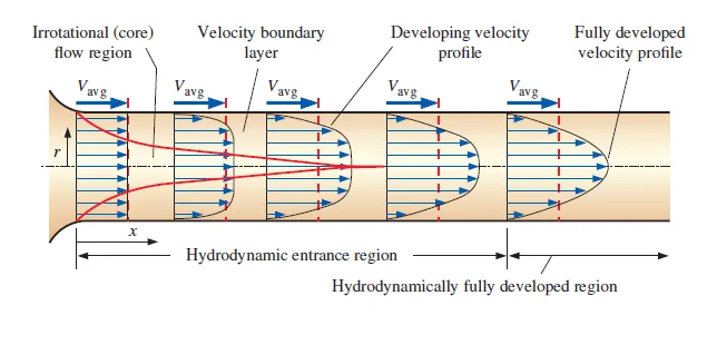
The fluid velocity changes from zero to wall and becomes maximum at the center. In fluid flow, it is preferred to take average velocity because it remains constant when the flow is incompressible and the cross-sectional area is constant.
Hagen-Poiseuille equation
The assumptions of the equations are that the fluid is incompressible and Newtonian, the flow is laminar through a pipe of the constant cross-section of length that is longer than the diameter, and there is no acceleration of the fluid in the pipe. The Hagen-Poiseuille equation os written as
Pressure drop for the fluid in the laminar flow `Delta p = (32*mu*v*L)/D^2`
The velocity profile remains unchanged in the hydrodynamically fully developed region, the shear stress at the wall also remains unchanged.
Avarage Velocity `v_(avg) = (R_e*mu)/(rho*D)`
Maximum Velocity `v_(max) = 2*v_(avg)`
Kinematic pressure `DeltaP_k = (DeltaP)/(rho)`
Shear stress `tau = (2*mu*v_max*R)/(r^2)`
BODY OF CONTENT
At first let us define the blockMeshDict file using matlab
clear all
close all
clc
%inputs
d = 0.01
r = d/2;
%Reynolds number
r_e = 2100;
%Density
rho = 1000
%length
l_e = 0.06*r_e*d
l = l_e+0.5*(l_e);
%Kinematic viscosity
nu = 8.9e-7;
%Dynamic viscosity
mu = nu*rho
%Wedge angle
theta = 2;

v_avg = (r_e*nu)/d
v_max = 2*v_avg
%Dynamic pressure
dp = (32*mu*v_avg*l_e)/(d^2)
%Kinematic pressure
dp_k = dp/rho;
f1 = fopen('blockMeshDict','w')
fprintf(f1,'/*------------------------------------*- C++ -*-------------------------------------*/')
fprintf(f1,'\n')
fprintf(f1,'  ===========              |')
fprintf(f1,'\n')
fprintf(f1,'   \\       /  F ield         |  OpenFOAM: The Open Source CFD Toolbox\n')
fprintf(f1,'    \\     /   O peration     |  Website:  https://openfoam.org\n')
fprintf(f1,'     \\   /    A nd           |  Version:  8\n')
fprintf(f1,'      \\ /     M anipulation  |\n')
fprintf(f1,'/*-----------------------------------------------------------------------------------*/\n')
fprintf(f1,'FoamFile\n')
fprintf(f1,'{\n')
fprintf(f1,'     version   2.0;\n')
fprintf(f1,'     format    ascii;\n')
fprintf(f1,'     class     dictionary;\n')
fprintf(f1,'     object    blockMeshDict;\n')
fprintf(f1,'}\n')
fprintf(f1,'// * * * * * * * * * * * * * * * * * * * * * * * * * * * * * * * * * * * * * * * * * * // \n\n')
fprintf(f1,'convertToMeters 1;\n\n')
fprintf(f1,'vertices\n')
fprintf(f1,'(\n')
fprintf(f1,'\t(0 0 0)\n')
fprintf(f1,'\t(%d %d %d)\n' ,   0 , r*cosd(theta/2), r*sind(theta/2))
fprintf(f1,'\t(%d %d %d)\n' ,   0 , r*cosd(theta/2), -r*sind(theta/2))
fprintf(f1,'\t(%d %d %d)\n' ,   l , 0, 0)
fprintf(f1,'\t(%d %d %d)\n' ,   l , r*cosd(theta/2), r*sind(theta/2))
fprintf(f1,'\t(%d %d %d)\n' ,   l , r*cosd(theta/2), -r*sind(theta/2))
fprintf(f1,');\n')
fprintf(f1,'blocks\n')
fprintf(f1,'(\n')
fprintf(f1,'\t hex(0 3 5 2 0 3 4 1) (200 20 1) simpleGrading (1 1 1)\n')
fprintf(f1,');\n')
fprintf(f1,'edges\n')
fprintf(f1,'(\n')
fprintf(f1,'\tarc  %d %d (%d %d %d)\n',1,2,0,r,0)
fprintf(f1,'\tarc  %d %d (%d %d %d)\n',4,5,l,r,0)
fprintf(f1,');\n')
fprintf(f1,'boundary\n')
fprintf(f1,'(\n')
fprintf(f1,'\tinlet\n')
fprintf(f1,'\t{\n')
fprintf(f1,'\t\ttype patch;\n')
fprintf(f1,'\t\tfaces\n')
fprintf(f1,'\t\t(\n')
fprintf(f1,'\t\t\t(0 1 2 0)\n')
fprintf(f1,'\t\t);\n')
fprintf(f1,'\t}\n')
fprintf(f1,'\toutlet\n')
fprintf(f1,'\t{\n')
fprintf(f1,'\t\ttype patch;\n')
fprintf(f1,'\t\tfaces\n')
fprintf(f1,'\t\t(\n')
fprintf(f1,'\t\t\t(3 4 5 3)\n')
fprintf(f1,'\t\t);\n')
fprintf(f1,'\t}\n')
fprintf(f1,'\tfront\n')
fprintf(f1,'\t{\n')
fprintf(f1,'\t\ttype wedge;\n')
fprintf(f1,'\t\tfaces\n')
fprintf(f1,'\t\t(\n')
fprintf(f1,'\t\t\t(0 3 4 1)\n')
fprintf(f1,'\t\t);\n')
fprintf(f1,'\t}\n')
fprintf(f1,'\tback\n')
fprintf(f1,'\t{\n')
fprintf(f1,'\t\ttype wedge;\n')
fprintf(f1,'\t\tfaces\n')
fprintf(f1,'\t\t(\n')
fprintf(f1,'\t\t\t(0 2 5 3)\n')
fprintf(f1,'\t\t);\n')
fprintf(f1,'\t}\n')
fprintf(f1,'\tTop\n')
fprintf(f1,'\t{\n')
fprintf(f1,'\t\ttype wall;\n')
fprintf(f1,'\t\tfaces\n')
fprintf(f1,'\t\t(\n')
fprintf(f1,'\t\t\t(1 4 5 2)\n')
fprintf(f1,'\t\t);\n')
fprintf(f1,'\t}\n')
fprintf(f1,'\taxis\n')
fprintf(f1,'\t{\n')
fprintf(f1,'\t\ttype empty;\n')
fprintf(f1,'\t\tfaces\n')
fprintf(f1,'\t\t(\n')
fprintf(f1,'\t\t\t(0 3 3 0)\n')
fprintf(f1,'\t\t);\n')
fprintf(f1,'\t}\n')
fprintf(f1,');\n')
fprintf(f1,'mergePatchPairs\n')
fprintf(f1,'(\n')
fprintf(f1,');\n')
fprintf(f1,'// * * * * * * * * * * * * * * * * * ** * * * * * * * * * * * * * * * * * * * * * * * * * * * // \n')
In the above program first we define the inputs and the given details that are required to solve the Hagen Poiseuille equation, thus we calculate all the necessary elements like average velocity, dynamic viscosity, kinematic viscosity, entrance length , total length, density, Reynold's number etc and we calculate the change in prtessure which results in the motion of the fluid inside the cylinder.
Then we define the blockMeshDict file using the file parsing technique. Using the fprintf command we print all the necessary vertices, boundary conditions in the file which after printing will appear as shown below
/*------------------------------------*- C++ -*-------------------------------------*\
  ===========                |
   \       /  F ield         |  OpenFOAM: The Open Source CFD Toolbox
    \     /   O peration     |  Website:  https://openfoam.org
     \   /    A nd           |  Version:  8
      \ /     M anipulation  |
\*-----------------------------------------------------------------------------------*/
FoamFile
{
     version   2.0;
     format    ascii;
     class     dictionary;
     object    blockMeshDict;
}
// * * * * * * * * * * * * * * * * * * * * * * * * * * * * * * * * * * * * * * * * * * //

convertToMeters 1;

vertices
(
	(0 0 0)
	(0 4.999238e-03 8.726203e-05)
	(0 4.999238e-03 -8.726203e-05)
	(1.890000e+00 0 0)
	(1.890000e+00 4.999238e-03 8.726203e-05)
	(1.890000e+00 4.999238e-03 -8.726203e-05)
);
blocks
(
	 hex(0 3 5 2 0 3 4 1) (200 20 1) simpleGrading (1 1 1)
);
edges
(
	arc  1 2 (0 5.000000e-03 0)
	arc  4 5 (1.890000e+00 5.000000e-03 0)
);
boundary
(
	inlet
	{
		type patch;
		faces
		(
			(0 1 2 0)
		);
	}
	outlet
	{
		type patch;
		faces
		(
			(3 4 5 3)
		);
	}
	front
	{
		type wedge;
		faces
		(
			(0 3 4 1)
		);
	}
	back
	{
		type wedge;
		faces
		(
			(0 2 5 3)
		);
	}
	Top
	{
		type wall;
		faces
		(
			(1 4 5 2)
		);
	}
	axis
	{
		type empty;
		faces
		(
			(0 3 3 0)
		);
	}
);
mergePatchPairs
(
);
// * * * * * * * * * * * * * * * * * ** * * * * * * * * * * * * * * * * * * * * * * * * * * * //
After that then we change the controldict file along with velocity and pressure file and the transport properties
/*--------------------------------*- C++ -*----------------------------------*\
  =========                 |
  \\      /  F ield         | OpenFOAM: The Open Source CFD Toolbox
   \\    /   O peration     | Website:  https://openfoam.org
    \\  /    A nd           | Version:  8
     \\/     M anipulation  |
\*---------------------------------------------------------------------------*/
FoamFile
{
    version     2.0;
    format      ascii;
    class       dictionary;
    location    "system";
    object      controlDict;
}
// * * * * * * * * * * * * * * * * * * * * * * * * * * * * * * * * * * * * * //

application     icoFoam;

startFrom       startTime;

startTime       0;

stopAt          endTime;

endTime         11;

deltaT          0.01;

writeControl    timeStep;

writeInterval   20;

purgeWrite      0;

writeFormat     ascii;

writePrecision  6;

writeCompression off;

timeFormat      general;

timePrecision   6;

runTimeModifiable true;


// ************************************************************************* //
Here in the controlDict file we change the end time and time step because we calculate the end time as the total length/average velocity here it is 1.89/0.186 which is approximately 11, thus we give the simulation end time as 11 seconds
Pressure file
/*--------------------------------*- C++ -*----------------------------------*\
  =========                 |
  \\      /  F ield         | OpenFOAM: The Open Source CFD Toolbox
   \\    /   O peration     | Website:  https://openfoam.org
    \\  /    A nd           | Version:  8
     \\/     M anipulation  |
\*---------------------------------------------------------------------------*/
FoamFile
{
    version     2.0;
    format      ascii;
    class       volScalarField;
    object      p;
}
// * * * * * * * * * * * * * * * * * * * * * * * * * * * * * * * * * * * * * //

dimensions      [0 2 -2 0 0 0 0];

internalField   uniform 0;

boundaryField
{
    inlet
    {
        type            zeroGradient;
    }
    outlet
    {
        type            fixedValue;
        value           uniform 0.0671;
    }

    Top
    {
        type            zeroGradient;
    }

    front
    {
        type            wedge;
    }
    back
    {
        type            wedge;
    }
    axis
    {
        type            empty;
    }
}

// ************************************************************************* //
Here in the pressure file we give value for the outlet pressure which is the kinematic pressure that is 0.0671
Velocity file
/*--------------------------------*- C++ -*----------------------------------*\
  =========                 |
  \\      /  F ield         | OpenFOAM: The Open Source CFD Toolbox
   \\    /   O peration     | Website:  https://openfoam.org
    \\  /    A nd           | Version:  8
     \\/     M anipulation  |
\*---------------------------------------------------------------------------*/
FoamFile
{
    version     2.0;
    format      ascii;
    class       volVectorField;
    object      U;
}
// * * * * * * * * * * * * * * * * * * * * * * * * * * * * * * * * * * * * * //

dimensions      [0 1 -1 0 0 0 0];

internalField   uniform (0.1869 0 0);

boundaryField
{
    inlet
    {
        type            fixedValue;
        value           uniform (0.1869 0 0);
    }
     outlet
    {
        type            zeroGradient;

    }


    Top
    {
        type            noSlip;
    }

    front
    {
        type            wedge;
    }

    back
    {
        type            wedge;
    }
}

// ************************************************************************* //
Here the velocity is the average velocity = 0.1869 m/s.
Transport properties
/*--------------------------------*- C++ -*----------------------------------*\
  =========                 |
  \\      /  F ield         | OpenFOAM: The Open Source CFD Toolbox
   \\    /   O peration     | Website:  https://openfoam.org
    \\  /    A nd           | Version:  8
     \\/     M anipulation  |
\*---------------------------------------------------------------------------*/
FoamFile
{
    version     2.0;
    format      ascii;
    class       dictionary;
    location    "constant";
    object      transportProperties;
}
// * * * * * * * * * * * * * * * * * * * * * * * * * * * * * * * * * * * * * //

nu              [0 2 -1 0 0 0 0] 8.9e-7;


// ************************************************************************* //
In the transport properties file we change the value of kinematic viscosity nu from 0.1 to the kinematic viscosity of water which is 8.9e-7.
Program to find shear stress analytically
clear all
close all
clc
r_c = 0.005
r = linspace(0,r_c,200)
mu = 8.9e-4
v_max = 0.3738
for i =1:length(r)
    tau(i) = 2*mu*v_max*(r(i)/(r_c)^2)
end
plot(r,tau)
xlabel('radius')
ylabel('shear stress')
In the above program we calculate the shear stress using the equation `tau = (2*mu*v_max*R)/(r^2)`
OUTPUT
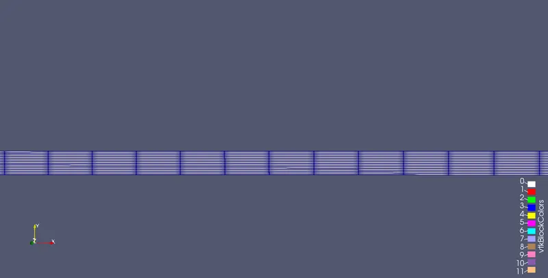
The above image is the paraview representation of the surface with edges.
Velocity distribution result by applying initial and boundary condition
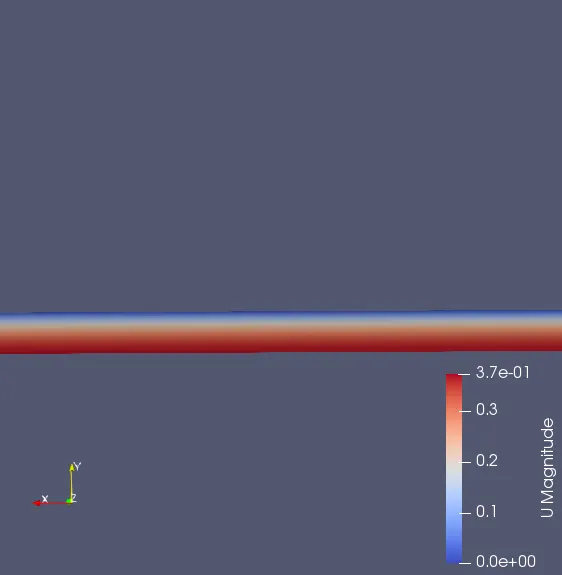
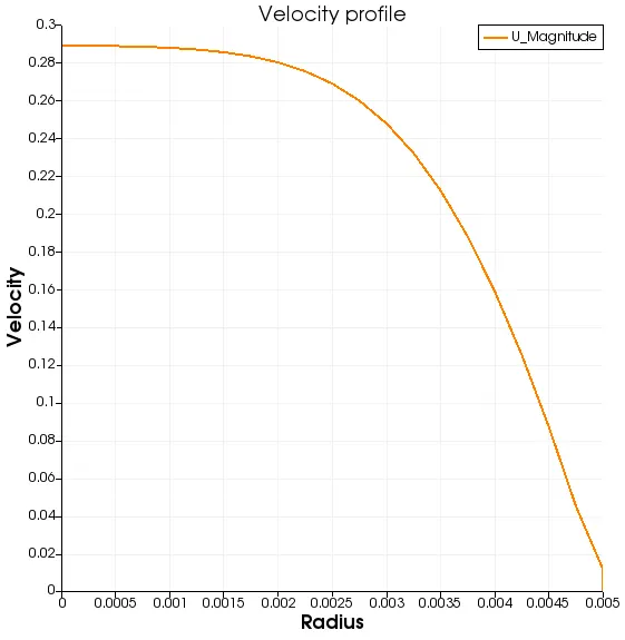
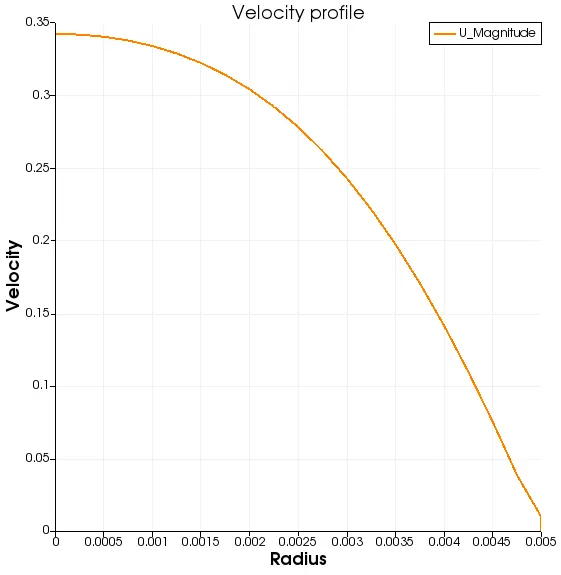
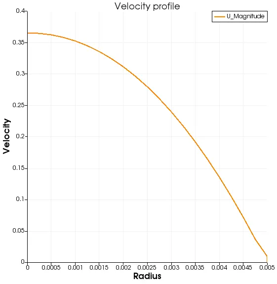
Velocity profile at varying x axis
At 0.2 m from inlet
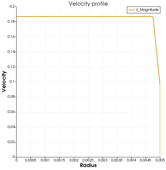
At x = 0.6
At x = 0.8
At x = 1.4
At x =1.6
From the above plots we can see that the velocity is maximum at the middle of the boundary layer and also after reaching the entrance length the flow becomes fully developed and the velocity doesn't change after that.
Let us compare the analytical one that we calculated through matlab and the one which we got through paraview
Hydrodynamic entrance length l_e (Numerical)= 1.2600
Hydrodynamic entrance length l_e (Analytical) = 1.246
v_max (numerical) =0.3738
v_max (analytical) = 0.3653
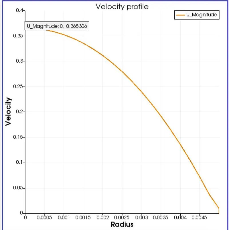
Now we find the shear stress first numerically using matlab program and then through paraview.
clear all
close all
clc
r_c = 0.005
r = linspace(0,r_c,200)
mu = 8.9e-4
v_max = 0.3738
for i =1:length(r)
    tau(i) = 2*mu*v_max*(r(i)/(r_c)^2)
end
plot(r,tau)
xlabel('radius')
ylabel('shear stress')
OUTPUT
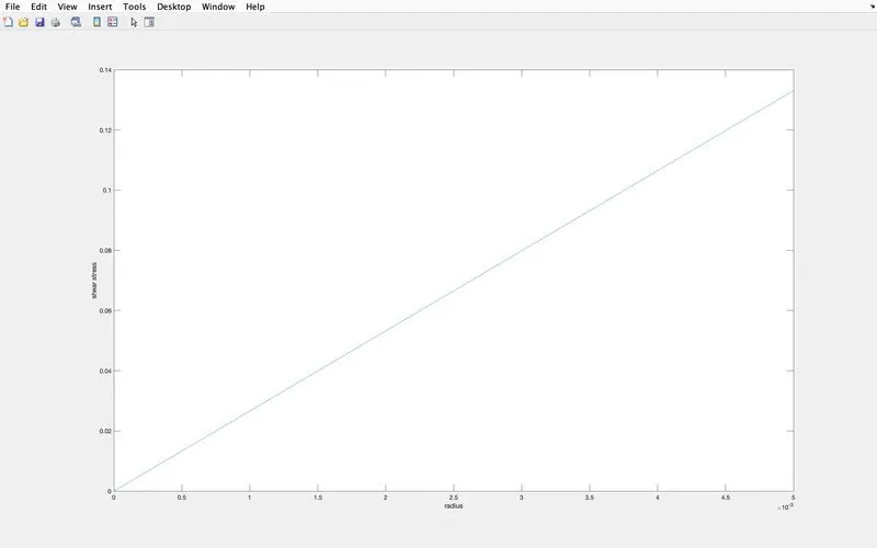
Then we find the shear stress using the equation `tau = mu*(du)/(dy)`and apply it on the paraview and we created a shear stress plot using paraview
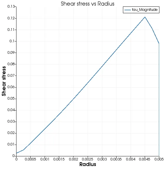
In the above plot we can conclude that shear stress is maximum at the walls and it reduces while moving away from it.As we can see that shear stress increases along the radius i.e shear stress is 0 at the centre of the pipe and it is maximum at the walls.
By comparing these two we can cocnlude the same that as radius increases shear stress increases.
RESULTS
| Maximum Velocity (m/s) |
Pressure Loss (Pa) |
Maximum Stress |
| Numerical Results | 0.3653 | 0.0665 | 0.13279 |
| Theoretical Results | 0.3738 | 0.0671 | 0.1283 |
Thus the program to simulate an axi-symmetric flow by applying the wedge boundary condition is successfully completed and the results are noted as per the requirement