Week 11 - Simulation of Flow through a pipe in OpenFoam
Simulation of flow through a pipe using OpenFOAM
Aim: To simulate an axisymmetric flow by using the wedge boundary condition.
Objectives:
1. To perform a transient/steady state simulation.
2. To validate the results with Hagen-Poiseuille's equation for the fully developed flow.
3. To write a code in Matlab to generate the blockMeshDict file.
Theory:
Hagen-Poiseuille's equation:
In nonideal fluid dynamics, Hagen-Poiseuille's equation also known as Hagen-Poiseuille's law or Poiseuille's equation is a physical law that gives the pressure drop in an incompressible and Newtonian fluid in laminar flow flowing through a long cylindrical pipe of a constant cross-section.
Mathematically,
`Delta P=(32 mu V_(avg) L)/D^2`
where,
`Delta P`=pressure difference between the two ends
`mu`=dynamic viscosity
`V_(avg)`=average velocity
`L`=lenghth of pipe
`D`=diameter of pipe
Assumptions:
1. The flow is axisymmetric: the flow is symmetric to the axis of the pipe.
2. Renoylds no. (Re)=2100 (laminar flow)
3. Fluid is water,density `,rho_(water)`=997 `(kg)/m^3`
4. Dia of pipe, D=0.02 m; Radius, R=0.0.1 m
5.Dynamic viscosity,`mu=8.90 *10^(-4) pa-s`at about `25 ^o c`
6. Wedge angle,`theta=3^o`
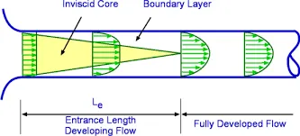
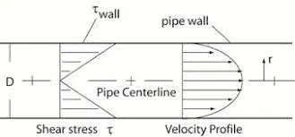
Formula used:
Avg velocity,`V_(avg) =(Re*mu)/(rho .D)`
Maximum velocity,`V_max=2*V_(avg)`
kinematic viscosity,`nu=mu/rho`=`8.93*e^-7`
kinematic pressure drop=`Delta P/rho`=0.018 `m^2/s^2`
shear stress,`tau=mu*(du)/(dy)`
Procedure: using WSL (openFoam for Windows 10 )
1. Open the terminal by just running the Ubuntu app.
2. Type $FOAM_TUTORIALS or TUT in the terminal window.
3. We have to solve incompressible flow simulation for this problem so select incompressible directory by typing ‘cd incompressible’ and then again type 'ls' to explore folders in incompressible folders.
4. For this particular case we need a solver for laminar-viscous flow. So here we have to choose ‘icoFoam’.Therefore, we will select icoFoam folder by typing ‘cd icoFoam’ and by typing ‘ls’ we explore this folder in the terminal.
5.Here, we have, again two options, cavity and elbow. They both are part of the icoFoam solver and cavity section is used to create required domain and black mesh so select the ‘cavity’ folder.By typing ‘cd cavity’ and then again typing 'ls' to explore folders in cavity folder.(0,constant,system)
6. We are not going to make any changes here in the tutorial section. So, we are going to copy this cavity folder using the ‘cp -r cavity’ command and paste it into OpenFOAM run folder by typing ‘cp -r cavity $FOAM_RUN/pipeflow’.
7. Then open the run folder by typing ‘cd $FOAM_RUN’. where we can see the pipeflow file.
8.Type 'ls' to explore folders in pipeflow file.(0,constant,system).
9.We have to open the system folder by typing 'cd system'.There are 4 script files in the system folder(blockMeshDict controlDict fvSchemes fvSolution )and by opening blockMeshDict we can create domain and provide the required specification for block mesh.
10.Type notepad.exe blockMeshDict to open the blockMeshDict .We have to replace the file with the file created by using MatLab and save it.
blockMeshDict file is used for creating geometry, generating mesh, and defining boundary conditions. The following procedures need to be followed in creating geometry in blockMesh.
Let us consider creating the geometry as shown in the figure below,
MatLab program to create blockMeshDict file:
clear all
close all
clc

%program to create blockMeshDict file for pipe flow

%inputs
Re=2100 %Reynolds number;
L=2.7 % length(m);
D=0.02 %dia(m);
mu=8.90e-4 % dynamic viscosity(pa-s);
theta=3 %wedge angle(degree);
R=D/2 % radius(m);
Le=0.06*Re*D %entrance length;

%determining the vertices of wedge
v0=[0,0,0];
v1=[0,(R*cosd(theta/2)),(R*sind(theta/2))];
v2=[0,(R*cosd(theta/2)),(-R*sind(theta/2))];
v3=[L,0,0];
v4=[L,(R*cosd(theta/2)),(R*sind(theta/2))];
v5=[L,(R*cosd(theta/2)),(-R*sind(theta/2))];


f1=fopen('blockMeshDict.txt','w')
fprintf(f1,'/*--------------------------------*- MATLAB -*----------------------------------*');
fprintf(f1,'\n=========                  ');
fprintf(f1,'\n  \\       /  F ield         | OpenFOAM: The Open Source CFD Toolbox');
fprintf(f1,'\n   \\     /   O peration     | Website:  https://openfoam.org');
fprintf(f1,'\n    \\   /    A nd           | Version:  10');
fprintf(f1,'\n     \\ /     M anipulation  |');
fprintf(f1,'\n*---------------------------------------------------------------------------*/');
fprintf(f1,'\nFoamFile');
fprintf(f1,'\n{');
fprintf(f1,'\nformat      ascii;');
fprintf(f1,'\nclass       dictionary;');
fprintf(f1,'\nobject      blockMeshDict;');
fprintf(f1,'\n}');
fprintf(f1,'\n// * * * * * * * * * * * * * * * * * * * * * * * * * * * * * * * * * * * * * //');

fprintf(f1,'\n\nconvertToMeters 1;');
%vertices
fprintf(f1,'\n\nvertices');
fprintf(f1,'\n(');
fprintf(f1,'\n(%f %f %f)//point0',v0(1),v0(2),v0(3));
fprintf(f1,'\n(%f %f %f)//point1',v1(1),v1(2),v1(3));
fprintf(f1,'\n(%f %f %f)//point2',v2(1),v2(2),v2(3));
fprintf(f1,'\n(%f %f %f)//point3',v3(1),v3(2),v3(3));
fprintf(f1,'\n(%f %f %f)//point4',v4(1),v4(2),v4(3));
fprintf(f1,'\n(%f %f %f)//point5',v5(1),v5(2),v5(3));
fprintf(f1,'\n);');
fprintf(f1,'\nblocks');
fprintf(f1,'\n(');
fprintf(f1,'\n  hex (0 3 5 2 0 3 4 1) (200 20 1) simpleGrading (1 1 1)');
fprintf(f1,'\n);');
%edges
fprintf(f1,'\n %s \n','edges');
fprintf(f1,'%s \n','(');
fprintf(f1,'\n arc 1 2 (%f %f %f)',0,R,0);
fprintf(f1,'\n arc 4 5 (%f %f %f)',L,R,0);
fprintf(f1,'\n);');

%boundary

fprintf(f1,'\nboundary');
fprintf(f1,'\n(');
fprintf(f1,'\n    inlet');
fprintf(f1,'\n    {');
fprintf(f1,'\n	type patch;');
fprintf(f1,'\n	faces');
fprintf(f1,'\n	(');
fprintf(f1,'\n	(0 1 2 0)');
fprintf(f1,'\n);');
fprintf(f1,'\n    }');
fprintf(f1,'\n    outlet');
fprintf(f1,'\n    {');
fprintf(f1,'\n	type patch;');
fprintf(f1,'\n	faces');
fprintf(f1,'\n	(');
fprintf(f1,'\n	(3 5 4 3)');
fprintf(f1,'\n);');
fprintf(f1,'\n    }');
%wall
fprintf(f1,'\n %s \n','wall')
fprintf(f1,'%s \n','{')
fprintf(f1,'\n	type wall;');
fprintf(f1,'\n	faces');
fprintf(f1,'\n	(');
fprintf(f1,'\n	(1 4 5 2)');
fprintf(f1,'\n);');
fprintf(f1,'\n    }');
%frontand back
fprintf(f1,'\n %s \n','front')
fprintf(f1,'%s \n','{')
fprintf(f1,'\n	type wedge;');
fprintf(f1,'\n	faces');
fprintf(f1,'\n	(');
fprintf(f1,'\n	(0 3 4 1)');
fprintf(f1,'\n);');
fprintf(f1,'\n    }');
fprintf(f1,'\n %s \n','back')
fprintf(f1,'%s \n','{')
fprintf(f1,'\n	type wedge;');
fprintf(f1,'\n	faces');
fprintf(f1,'\n	(');
fprintf(f1,'\n	(0 2 5 3)');
fprintf(f1,'\n);');
fprintf(f1,'\n    }');
fprintf(f1,'\n %s \n','axis')
fprintf(f1,'%s \n','{')
fprintf(f1,'\n	type empty;');
fprintf(f1,'\n	faces');
fprintf(f1,'\n	(');
fprintf(f1,'\n	(0 3 3 0)');
fprintf(f1,'\n);');
fprintf(f1,'\n    }');
fprintf(f1,'\n);');

fprintf(f1,'\n %s \n','mergePatchPairs')
fprintf(f1,'\n(');
fprintf(f1,'\n);');
fprintf(f1,'\n // ************************************************************************* //');
blockMeshDict:
/*--------------------------------*- MATLAB -*----------------------------------*
=========
  \       /  F ield         | OpenFOAM: The Open Source CFD Toolbox
   \     /   O peration     | Website:  https://openfoam.org
    \   /    A nd           | Version:  10
     \ /     M anipulation  |
*---------------------------------------------------------------------------*/
FoamFile
{
format      ascii;
class       dictionary;
object      blockMeshDict;
}
// * * * * * * * * * * * * * * * * * * * * * * * * * * * * * * * * * * * * * //

convertToMeters 1;

vertices
(
(0.000000 0.000000 0.000000)//point0
(0.000000 0.009997 0.000262)//point1
(0.000000 0.009997 -0.000262)//point2
(2.700000 0.000000 0.000000)//point3
(2.700000 0.009997 0.000262)//point4
(2.700000 0.009997 -0.000262)//point5
);
blocks
(
  hex (0 3 5 2 0 3 4 1) (200 20 1) simpleGrading (1 1 1)
);
 edges
(

 arc 1 2 (0.000000 0.010000 0.000000)
 arc 4 5 (2.700000 0.010000 0.000000)
);
boundary
(
    inlet
    {
	type patch;
	faces
	(
	(0 1 2 0)
         );
    }
    outlet
    {
	type patch;
	faces
	(
	(3 5 4 3)
         );
     }
 wall
      {

	type wall;
	faces
	(
	(1 4 5 2)
        );
        }

 front
   {

	type wedge;
	faces
	(
	(0 3 4 1)

         );
    }
back
   {

	type wedge;
	faces
	(

	(0 2 5 3)
         );
    }
 axis
  {

	type empty;
	faces
	(
	(0 3 3 0)
        );
    }
);
 mergePatchPairs
(
);
 // ************************************************************************* //
11. The next step is to navigate to the controlDict folder and specify the simulation time as 10 seconds and time step deltaT as 1e-3 at interval 100.
controlDict
/*--------------------------------*- C++ -*----------------------------------*\
  =========                 |
  \\      /  F ield         | OpenFOAM: The Open Source CFD Toolbox
   \\    /   O peration     | Website:  https://openfoam.org
    \\  /    A nd           | Version:  10
     \\/     M anipulation  |
\*---------------------------------------------------------------------------*/
FoamFile
{
    format      ascii;
    class       dictionary;
    location    "system";
    object      controlDict;
}
// * * * * * * * * * * * * * * * * * * * * * * * * * * * * * * * * * * * * * //

application     icoFoam;

startFrom       startTime;

startTime       0;

stopAt          endTime;

endTime         10;

deltaT         1e-3;

writeControl    timeStep;

writeInterval  100;

purgeWrite      0;

writeFormat     ascii;

writePrecision  6;

writeCompression off;

timeFormat      general;

timePrecision   6;

runTimeModifiable true;


// ************************************************************************* //
12.Making changes in boundary condition and p and U textfile in 0 folder.
p:
/*--------------------------------*- C++ -*----------------------------------*\
  =========                 |
  \\      /  F ield         | OpenFOAM: The Open Source CFD Toolbox
   \\    /   O peration     | Website:  https://openfoam.org
    \\  /    A nd           | Version:  10
     \\/     M anipulation  |
\*---------------------------------------------------------------------------*/
FoamFile
{
    format      ascii;
    class       volScalarField;
    object      p;
}
// * * * * * * * * * * * * * * * * * * * * * * * * * * * * * * * * * * * * * //

dimensions      [0 2 -2 0 0 0 0];

internalField   uniform 0;
boundaryField
{
    inlet
    {
        type            zeroGradient;
    }

    outlet
    {
        type            fixedValue;
        value           uniform 0.018;
    }

   wall
    {
         type           zeroGradient;
    }

    front
    {
        type            wedge;
    }

    back
    {
        type            wedge;
    }

     axis
    {
        type            empty;
    }


}

// ************************************************************************* //
U:
/*--------------------------------*- C++ -*----------------------------------*\
  =========                 |
  \\      /  F ield         | OpenFOAM: The Open Source CFD Toolbox
   \\    /   O peration     | Website:  https://openfoam.org
    \\  /    A nd           | Version:  10
     \\/     M anipulation  |
\*---------------------------------------------------------------------------*/
FoamFile
{
    format      ascii;
    class       volVectorField;
    object      U;
}
// * * * * * * * * * * * * * * * * * * * * * * * * * * * * * * * * * * * * * //

dimensions      [0 1 -1 0 0 0 0];

internalField   uniform (0.0937 0 0);

boundaryField
{
    inlet
    {
        type             fixedValue;
        value            uniform (0.0937 0 0);
    }

    outlet
    {
        type           zeroGradient;

    }

    wall
    {
         type           noSlip;
    }

    front
    {
        type            wedge;
    }

    back
    {
        type            wedge;
    }

     axis
    {
        type            empty;
    }

}

// ************************************************************************* //
13.Making changes in constant folder the value of nu and save it.
/*--------------------------------*- C++ -*----------------------------------*\
  =========                 |
  \\      /  F ield         | OpenFOAM: The Open Source CFD Toolbox
   \\    /   O peration     | Website:  https://openfoam.org
    \\  /    A nd           | Version:  10
     \\/     M anipulation  |
\*---------------------------------------------------------------------------*/
FoamFile
{
    format      ascii;
    class       dictionary;
    location    "constant";
    object      physicalProperties;
}
// * * * * * * * * * * * * * * * * * * * * * * * * * * * * * * * * * * * * * //

nu              [0 2 -1 0 0 0 0] 8.93e-7;


// ************************************************************************* //
14.Type 'checkMesh' to check the blockMesh.
15. Type 'icoFoam' to run the solver.
16. Now, view the results in ParaView by using the ‘paraFoam’ command.
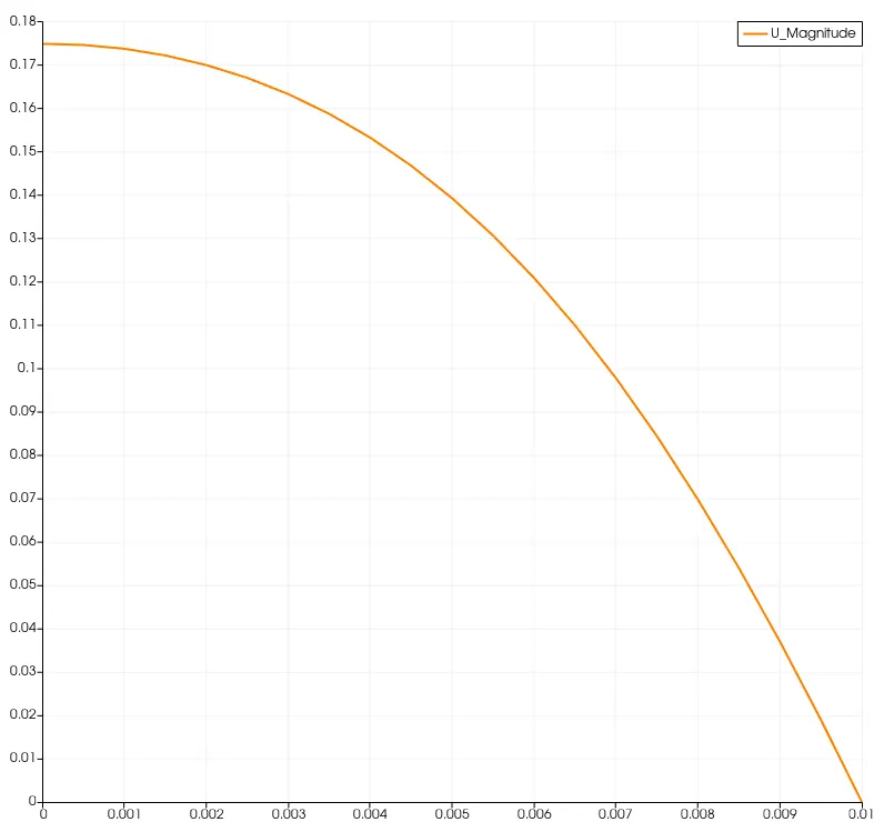
Velocity profile at x=2.6 m
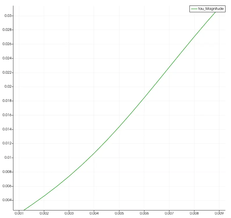
shear stress profile at x=2.6m
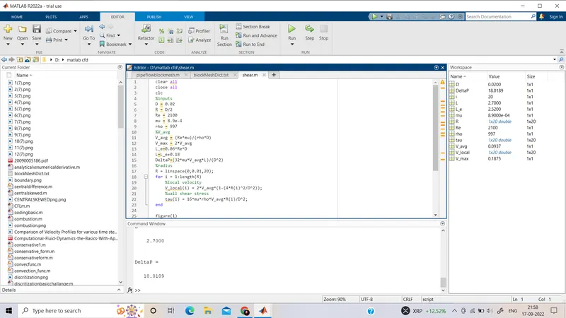
Analytical solution using MatLab:
clear all
close all
clc
%inputs
D = 0.02
R = D/2
Re = 2100
mu = 8.9e-4
rho = 997
%V_avg
V_avg = (Re*mu)/(rho*D)
V_max = 2*V_avg
L_e=0.06*Re*D
L=L_e+0.18
DeltaP=(32*mu*V_avg*L)/(D^2)
%radius
R = linspace(0,0.01,20);
for i = 1:length(R)
    %local velocity
    V_local(i) = 2*V_avg*(1-(4*R(i)^2/D^2));
    %wall shear stress
    tau(i) = 16*mu*rho*V_avg*R(i)/D^2;
end

figure(1)
plot(R,V_local)
xlabel('Radius')
ylabel('local velocity')
legend('analytical velocity profile')
figure(2)
plot(R,tau)
xlabel('Radius')
ylabel('wall shear stress')
legend('analytical wall shear stress profile')
D =
0.0200 m
R =
0.0100 m
Re =
2100
mu =
8.9000e-04 pa-s
rho =
997 `m^2`
V_avg =
0.0937 `m^2`
V_max =
0.1875 `m^2`
L_e =
2.5200 m
L =
2.7000 m
DeltaP =
18.0189 pa
where,L_e=hydro-dynamic length
L=total length
Validation of hydro-dynamic length with the numerical result: after passing Le i.e. x=2.52 m the flow will fully develop
velocity profile at x=0.01 m
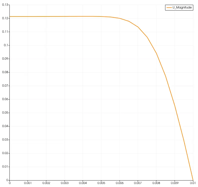
velocity profile at x=2.5 m
velocity profile at x=2.6 m
Validation of the fully developed flow velocity profile with its analytical profile:
The analytical profile generated using MatLab: (matches the velocity profile generated using OpenFOAM.)
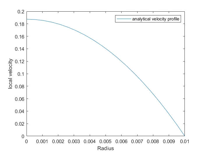
Validation of maximum velocity and pressure drop for fully developed flow:
`V_(avg )= (Re*mu)/(rho*D)`
`V_max=2*V_(avg)=0.1875 m^2`
By observing the graphs obtained in ParaView, we can say that when R=0 i.e. at the center there will be zero shear stress and maximum velocity. On the other hand, at R=0.01m i.e. at the circumference shear stress will be maximum and velocity will be zero.
Pressure drop:
`DeltaP=(32*mu*V_(avg)*L)/(D^2)`=18.0189 pa
Post-processing of Shear stress and validation of wall shear stress for fully developed flow:
using OpenFOAM:
using MATLAB:
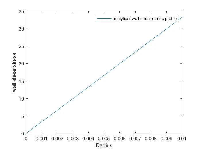
Conclusion: Simulation is performed successfully. It matches closely with the analytical solutions.