Week 11 - Simulation of Flow through a pipe in OpenFoam
Aim: Simulation of flow through pipe in OpenFOAM
Abstract:
The flow through a pipe is the case of internal flow. The surface is the duct in the case of air, it is a pipe in the case of water. The flow is driven because of the pressure difference created by the pumps, air handling units, fans, etc. They find their major application refrigeration and air conditioning industries.
The fluid velocity changes from zero to wall and becomes maximum at the center. In fluid flow, it is preferred to take average velocity because it remains constant when the flow is incompressible and the cross-sectional area is constant.
Assumptions
- The steady laminar incompressible flow of a fluid is taken.
• There is no velocity in the radial direction.
- .There is no acceleration since the flow is steady.
- Reynolds number for the laminar flow is 2100.
- Only the wedge shape of the pipe is considered because the flow is axis-symmetric.
- The equation governing the fluid flow is described by the Hagen-Poiseuille
Hagen Poiseuille equation
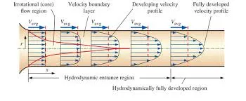
The assumptions of the equations are that the fluid is incompressible and Newtonian, the flow is laminar through a pipe of the constant cross-section of length that is longer than the diameter, and there is no acceleration of the fluid in the pipe.
The velocity profile remains unchanged in the hydrodynamically fully developed region, the shear stress at the wall also remains unchanged.
Hydrodynamically fully developed region `(del u(r,x))/(delx)` = 0 which means u = u(r)
Observation based on Hagen Poiseuille equation
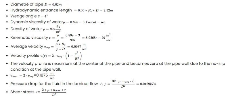
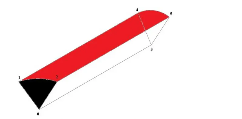
Matlab coding and script for blockMeshDict file:
/*--------------------------------*- C++ -*----------------------------------*\
========= |
\\ / F ield | OpenFOAM: The Open Source CFD Toolbox
\\ / O peration | Website: https://openfoam.org
\\ / A nd | Version: 9
\\/ M anipulation |
\*---------------------------------------------------------------------------*/
FoamFile
{
format ascii;
class dictionary;
object blockMeshDict;
}
// * * * * * * * * * * * * * * * * * * * * * * * * * * * * * * * * * * * * * //
convertToMeters 0.1;
vertices
(
(0.000000 0.0000 0.00000) // origin
(0.000000 0.009994 -0.000349) //1
(0.000000 0.009994 0.000349) //2
(2.520000 0.00000 0.000000)//3
2.520000 0.009994 -0.000349)//4
2.520000 0.009994 0.000349) //5
);
blocks
(
hex (0 1 2 0 3 4 5 3) (50 1 200) simpleGrading (0.4 1 1)
);
edges
(
arc 1 2 ( 0 0.01 0)
arc 4 5 (2.52 0.01 0)
);
boundary
(
axis
{
type empty;
faces
(
(0 3 3 0)
);
}
inlet
{
type patch;
faces
(
(0 1 2 0)
);
}
frontAndBack
{
type empty;
faces
(
(0 3 2 1)
(4 5 6 7)
);
}
);
mergePatchPairs
(
);
// ************************************************************************* //
/*--------------------------------*- C++ -*----------------------------------*\
========= |
\\ / F ield | OpenFOAM: The Open Source CFD Toolbox
\\ / O peration | Website: https://openfoam.org
\\ / A nd | Version: 9
\\/ M anipulation |
\*---------------------------------------------------------------------------*/
FoamFile
{
format ascii;
class dictionary;
location "system";
object controlDict;
}
// * * * * * * * * * * * * * * * * * * * * * * * * * * * * * * * * * * * * * //
application icoFoam;
startFrom startTime;
startTime 0;
stopAt endTime;
endTime 10;
deltaT 0.01;
writeControl timeStep;
writeInterval 10;
purgeWrite 0;
writeFormat ascii;
writePrecision 6;
writeCompression off;
timeFormat general;
timePrecision 6;
runTimeModifiable true;
// ************************************************************************* //
Transport properties:
/*--------------------------------*- C++ -*----------------------------------*\
========= |
\\ / F ield | OpenFOAM: The Open Source CFD Toolbox
\\ / O peration | Website: https://openfoam.org
\\ / A nd | Version: 9
\\/ M anipulation |
\*---------------------------------------------------------------------------*/
FoamFile
{
format ascii;
class dictionary;
location "constant";
object Transport properties;
}
// * * * * * * * * * * * * * * * * * * * * * * * * * * * * * * * * * * * * * //
nu [0 2 -1 0 0 0 0] 8.9268e-07;
// ************************************************************************* //
/*--------------------------------*- C++ -*----------------------------------*\
========= |
\\ / F ield | OpenFOAM: The Open Source CFD Toolbox
\\ / O peration | Website: https://openfoam.org
\\ / A nd | Version: 9
\\/ M anipulation |
\*---------------------------------------------------------------------------*/
FoamFile
{
format ascii;
class volScalarField;
object p;
}
// * * * * * * * * * * * * * * * * * * * * * * * * * * * * * * * * * * * * * //
dimensions [0 2 -2 0 0 0 0];
internalField uniform 0;
boundaryField
{
axis
{
type empty;
}
inlet
{
type zeroGradient;
}
Velocity:
/*--------------------------------*- C++ -*----------------------------------*\
========= |
\\ / F ield | OpenFOAM: The Open Source CFD Toolbox
\\ / O peration | Website: https://openfoam.org
\\ / A nd | Version: 9
\\/ M anipulation |
\*---------------------------------------------------------------------------*/
FoamFile
{
format ascii;
class volVectorField;
object U;
}
// * * * * * * * * * * * * * * * * * * * * * * * * * * * * * * * * * * * * * //
dimensions [0 1 -1 0 0 0 0];
internalField uniform (0 0 0);
boundaryField
{
movingWall
{
type fixedValue;
value uniform (10 0 0);
}
fixedWalls
{
type noSlip;
}
frontAndBack
{
type empty;
}
}
// ************************************************************************* //
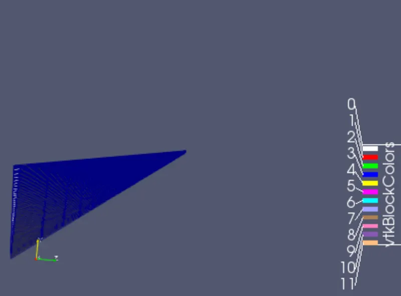
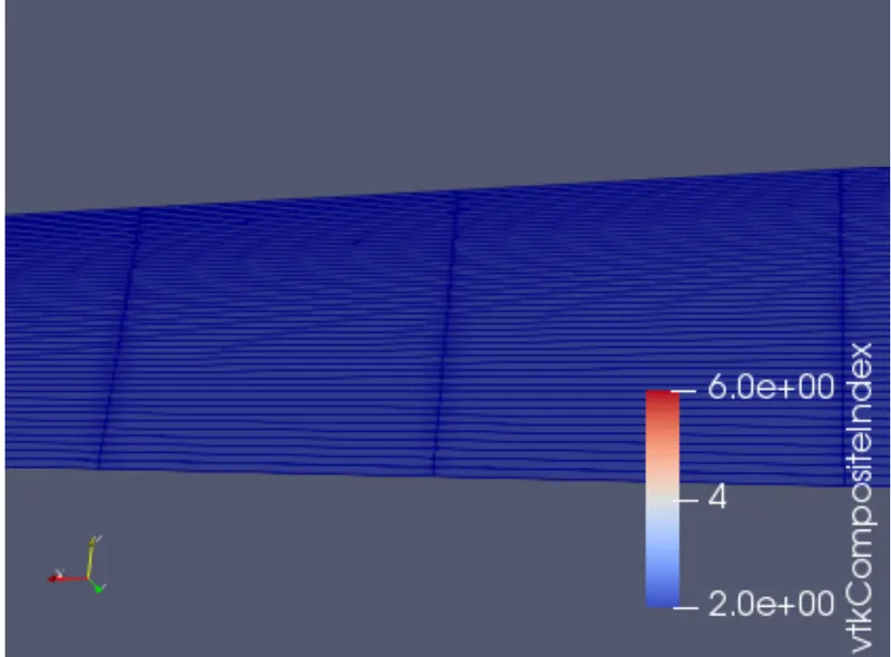
RESULTED GEOMETRY CREATED BY BLOCKMESHDICT:
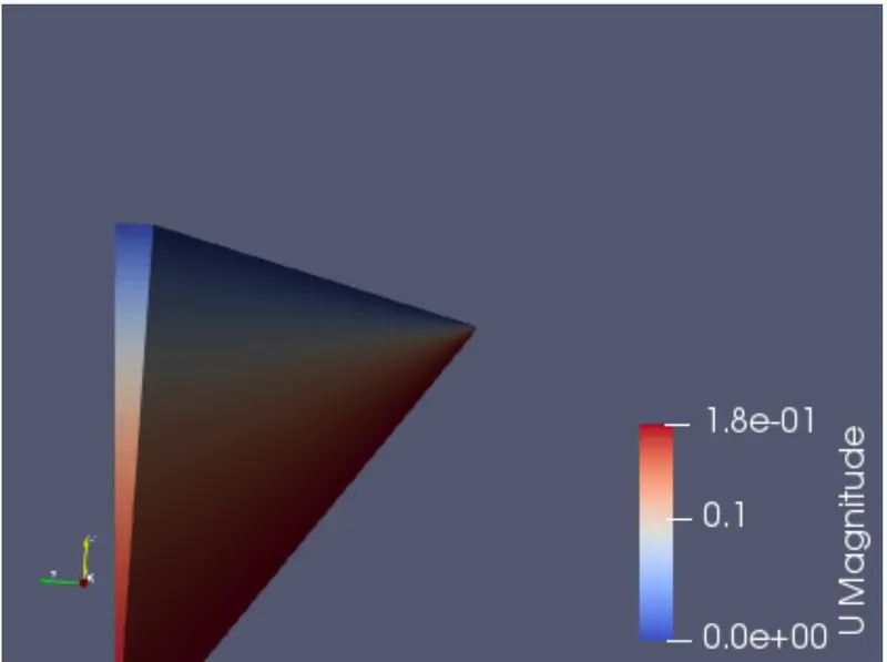
VELOCITY DISTRIBUTION RESULT BY APPLYING INITIAL AND BOUNDARY CONDITION
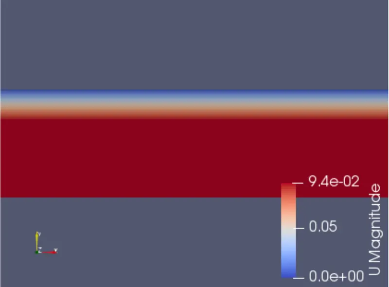
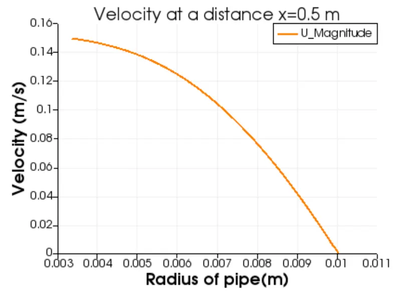
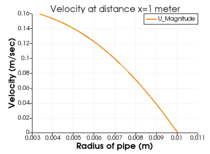
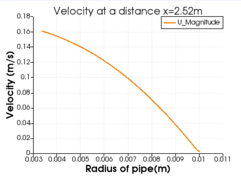
VELOCITY DISTRIBUTION ALONG THE LENGHT OF THE PIPE(FULLY DEVELOPED PROFILE)
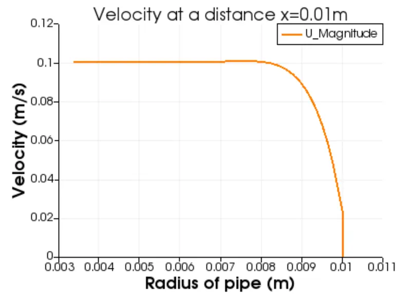
Simulation Graph:
velocity profile at the inlet
SHEAR STRESS:
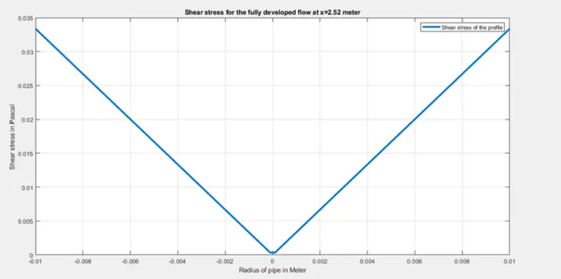
shear stress can be calculated `tau = mu((du)/(dr))`
where tau = shear stress
mu = viscosity
du/dr = velocity gradient
CALCULATING SHEAR STRESS NUMERICALLY
%%calculating shear stress
r = linspace(-0.01,0.01,100);
for i = 1:length(r)
tau(i) = 2*mu*u_max*abs(r(i)))/R^2;
end
plot(r,tau,'linewidth',3)
grid on
xlabel('Radius of pipe in meters')
ylabel(''shear stress in pascal)
legend('shear stress of profile')
SHEAR STRESS GRAPH FROM MATLAB
the open flow results are tabulated as:
Results Hagen poisueuille equation wedge angle 4
CFL number mean - 0.076
CFL number max - 0.304875
clock time - 141s
execution time - 114.63s
Umax 0.1875 0.16 m/s
CONCLUSION:
- The velocity profile is plotted at varying distances from the inlet of the pipe.
- The velocity at a distance-0.01 from the inlet seems to be slow and stable around the center of the pipe which shows that the velocity is gradually developing. It suddenly becomes zero at the wall because of the no slip condition.
- The velocity profile at a distance of -0.5 -1 -2.52 is parabolic in nature because the velocity profile moves to the hydrodynamically fully developed region.
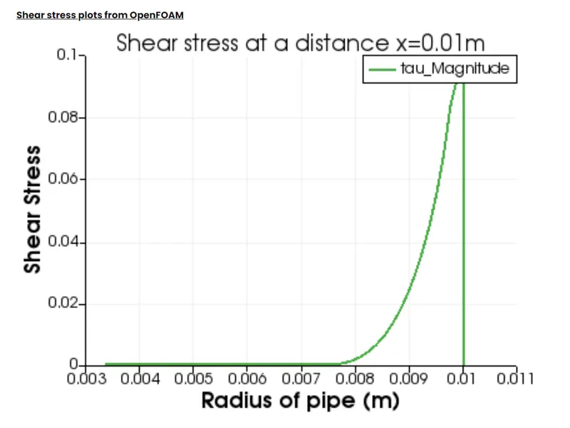
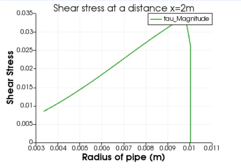
- The shear stress plot is plotted as shown above.
- The irregularities can be observed in the shear stress profile is because of the 'finite volume method. At nodes intersection the value of shear stress increases, this can be reduced by increasing the number of grid points which in turn will increase the computational time.
- The above table shows that the velocity profile calculated numerically is equal to the HP equation with an error of 0.0275.
- The simulation is done for wedge angle 4" but the values will be the same when the simulation is performed for the wedge angle 2", 3" since the flow is steady, incompressible.