Week 11 - Simulation of Flow through a pipe in OpenFoam
** Hagen Poiseuille Flow:
MATLAB Code to Generate BlockMesh file:
f1=fopen ('blockMeshDict','w')         % Create a text file with name "blockMeshDict"

fprintf(f1,'\nFoamFile')
fprintf(f1,'\n{')
fprintf(f1,'\n\tversion     2.0;')
fprintf(f1,'\n\tformat      ascii;')
fprintf(f1,'\n\tclass       dictionary;')
fprintf(f1,'\n\tobject      blockMeshDict;')
fprintf(f1,'\n}')
fprintf(f1,'\n//******************************//')
%% User inputs
l=1;
r=0.02;
Re=2100;
mu=8.90e-4;
theta=2;
rho=1000;
%%
le=0.06*Re*2*r;
lt=le+l;
v=Re*mu/(rho*2*r);
delta_p=32*mu*v*l/(4*r*r);
%% Caculate
fprintf(f1,'\nscale 1;')
fprintf(f1,'\nvertices')
fprintf(f1,'\n(')
fprintf(f1,'\n\t(0 0 0)')
fprintf(f1,'\n\t(0 %f %f)',r*cosd(theta),r*sind(theta))
fprintf(f1,'\n\t(0 %f %f)',r*cosd(theta),-r*sind(theta))
fprintf(f1,'\n\t(%f 0 0)',lt)
fprintf(f1,'\n\t(%f %f %f)',lt,r*cosd(theta),r*sind(theta))
fprintf(f1,'\n\t(%f %f %f)',lt,r*cosd(theta),-r*sind(theta))
fprintf(f1,'\n);')
fprintf(f1,'\nblocks')
fprintf(f1,'\n(')
fprintf(f1,'\nhex (0 3 5 2 0 3 4 1) (100 20 1) simpleGrading (1 0.1 1)')
fprintf(f1,'\n);')
fprintf(f1,'\nedges')
fprintf(f1,'\n(')
fprintf(f1,'\narc 1 2 (0 %f 0)',r)
fprintf(f1,'\narc 4 5 (%f %f 0)',lt,r)
fprintf(f1,'\n);')
%% Boundary conditions
fprintf(f1,'\nboundary')
fprintf(f1,'\n(')
fprintf(f1,'\n\t inlet')
fprintf(f1,'\n\t {')
fprintf(f1,'\n\t\t type patch;')
fprintf(f1,'\n\t\t faces')
fprintf(f1,'\n\t\t (')
fprintf(f1,'\n\t\t\t(0 1 2 0)')
fprintf(f1,'\n\t\t );')
fprintf(f1,'\n\t }')

fprintf(f1,'\n\t outlet')
fprintf(f1,'\n\t {')
fprintf(f1,'\n\t\t type patch;')
fprintf(f1,'\n\t\t faces')
fprintf(f1,'\n\t\t (')
fprintf(f1,'\n\t\t\t(3 5 4 3)')
fprintf(f1,'\n\t\t );')
fprintf(f1,'\n\t }')

fprintf(f1,'\n\t front')
fprintf(f1,'\n\t {')
fprintf(f1,'\n\t\t type wedge;')
fprintf(f1,'\n\t\t faces')
fprintf(f1,'\n\t\t (')
fprintf(f1,'\n\t\t\t(0 3 4 1)')
fprintf(f1,'\n\t\t );')
fprintf(f1,'\n\t }')

fprintf(f1,'\n\t back')
fprintf(f1,'\n\t {')
fprintf(f1,'\n\t\t type wedge;')
fprintf(f1,'\n\t\t faces')
fprintf(f1,'\n\t\t (')
fprintf(f1,'\n\t\t\t(0 2 5 3)')
fprintf(f1,'\n\t\t );')
fprintf(f1,'\n\t }')

fprintf(f1,'\n\t axis')
fprintf(f1,'\n\t {')
fprintf(f1,'\n\t\t type empty;')
fprintf(f1,'\n\t\t faces')
fprintf(f1,'\n\t\t (')
fprintf(f1,'\n\t\t\t(0 3 3 0)')
fprintf(f1,'\n\t\t );')
fprintf(f1,'\n\t }')

fprintf(f1,'\n\t pipeWall')
fprintf(f1,'\n\t {')
fprintf(f1,'\n\t\t type wall;')
fprintf(f1,'\n\t\t faces')
fprintf(f1,'\n\t\t (')
fprintf(f1,'\n\t\t\t(1 4 5 2)')
fprintf(f1,'\n\t\t );')
fprintf(f1,'\n\t }')
fprintf(f1,'\n);')

fprintf(f1,'\nmergePatchPairs')
fprintf(f1,'\n(')
fprintf(f1,'\n);')
fprintf(f1,'\n//******************************//')


fclose(f1)                    % Save the data into the file and close it
* Simulation Parameters:
#Entrance Length Calculation (Le):
Le=0.06*Re*2*r where Re is Raynold's number
Re=2100; r=0.02cm
Le= 5.04m
#Total Length of Pipe (Lt)= Le+1=6.04m
# Mean Velocity of Flow:
Re= Rho*Velocity*Lt/mu
For water,
Rho=1000 kg/m^3
mu=8.9e-4;
Hence velocity (v)= 0.0467 m/s
# Calculating simulation time:
ntime=Lt/velocity
ntime=129.267 seconds
Now making the similar changes in the controlDict file as well as U and p files
The following is the file
* ControlDict
FoamFile
{
    version     2.0;
    format      ascii;
    class       dictionary;
    location    "system";
    object      controlDict;
}
// * * * * * * * * * * * * * * * * * * * * * * * * * * * * * * * * * * * * * //

application     icoFoam;

startFrom       startTime;

startTime       0;

stopAt          endTime;

endTime         129.2670;

deltaT          0.05;

writeControl    timeStep;

writeInterval   100;

purgeWrite      0;

writeFormat     ascii;

writePrecision  6;

writeCompression off;

timeFormat      general;

timePrecision   6;

runTimeModifiable true;


// ************************************************************************* //
* U
FoamFile
{
    version     2.0;
    format      ascii;
    class       volVectorField;
    object      U;
}
// * * * * * * * * * * * * * * * * * * * * * * * * * * * * * * * * * * * * * //

dimensions      [0 1 -1 0 0 0 0];

internalField   uniform (0 0 0);

boundaryField
{
    inlet
    {
        type            fixedValue;
        value           uniform (0.046725 0 0);
    }

    outlet
    {
        type            zeroGradient;
    }

    front
    {
        type            wedge;
    }

	back
    {
        type            wedge;
    }

	axis
    {
        type            empty;
    }

	pipeWall
    {
        type            noSlip;
    }
}

// ************************************************************************* //
* p
dimensions      [0 2 -2 0 0 0 0];

internalField   uniform 0;

boundaryField
{
    inlet
    {
        type            zeroGradient;
    }

	outlet
    {
        type            fixedValue;
		value           uniform 0;
    }

	front
    {
        type            wedge;
    }

	back
    {
        type            wedge;
    }

	axis
    {
        type            empty;
    }

	pipeWall
    {
        type            zeroGradient;
    }

}

// ************************************************************************* //
## Formed Geometry and Mesh
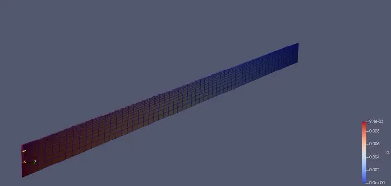
# Results:
1. Velocity Profiles
a. At Entrance
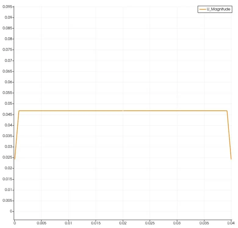
b. At x=0.1m
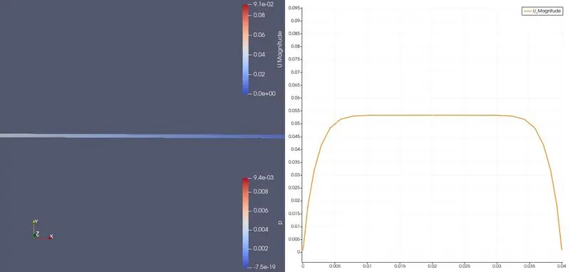
c. At x=0.25m
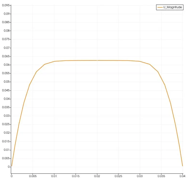
d At x=0.5m
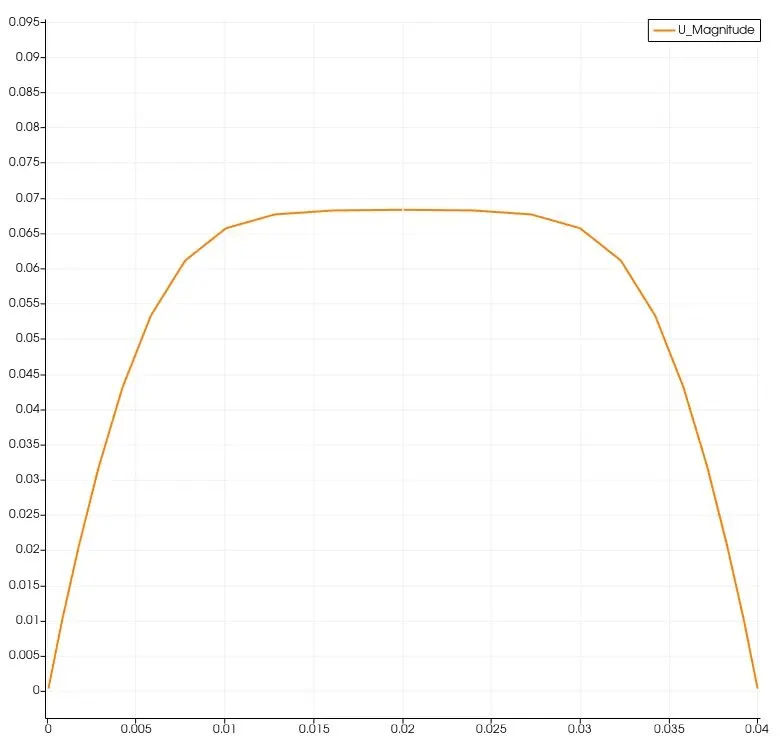
e. At x=0.75m
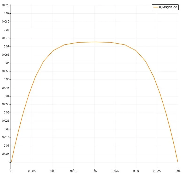
f. At x=1m
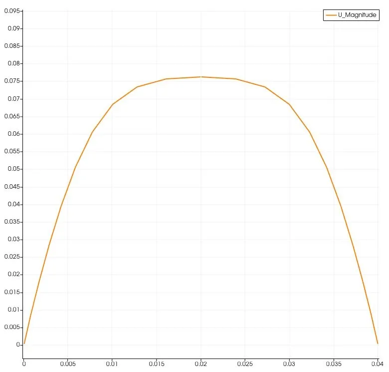
g. At x=2m
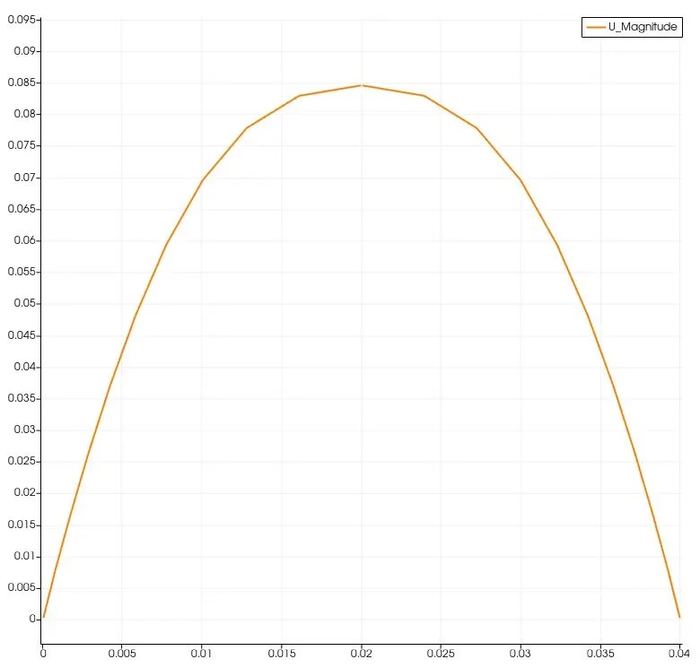
h. At x=4m
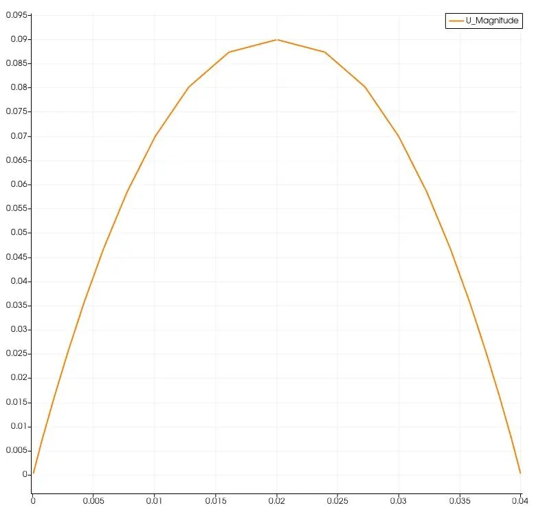
i. At x=5.04m
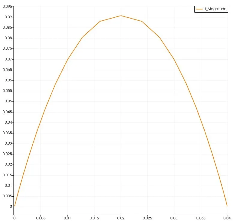
j. At exit
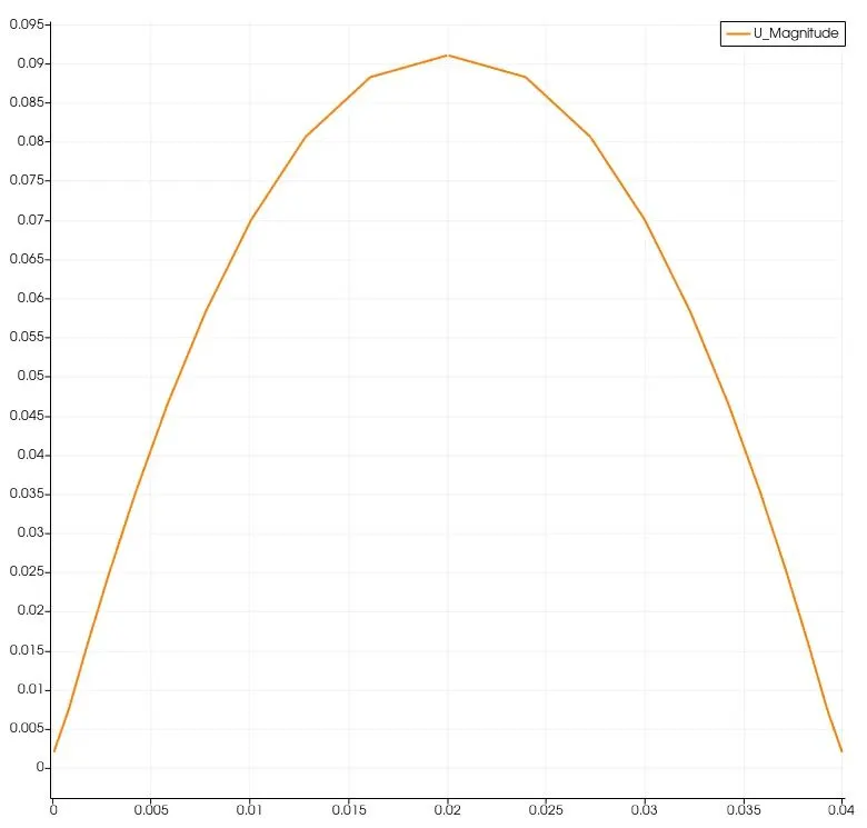
Hence at exit, maximum velocity is observed at centre of pipe (y=0.02m) and Vmax is 0.091m/s
* Pressure Drop in Fully Developed Region
The following graph is plotted for x=5.04m to x=6.04m
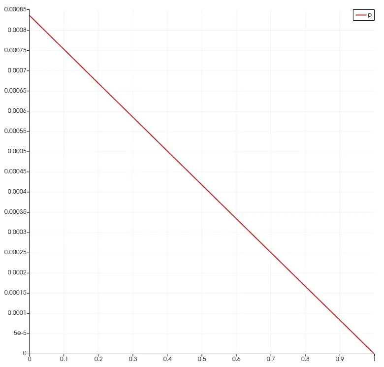
In above diagram, the guage pressure at exit of pipe is 0 atm (Exposed to atmosphere). And Pressure distribution is also correct since flow is exiting from outlet which has low pressure and the same is validated from equation
dp= 64*(v^2)*Lt/(Re*2*D)
dp is directly proportional to length of pipe (Lt). Hence a straight line relationship is expected.
* Shear Stress Distribution
The shear stress distribution along y direction in fully developed regime ( at x=5.05m)
The graph shown below is for y=0 to y=0.02m (only upper half of 2D pipe)
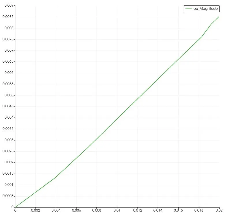
From the ideal shear stress distribution in the case of Hagen Poiseuille Flow, the plotted graph matches with analytical solution.