Week 11 - Simulation of Flow through a pipe in OpenFoam
WEEK 11 - SIMULATION OF FLOW THROUGH A PIPE IN OpenFOAM
AIM:
- To simulate an axi-symmetric flow by applying the wedge boundary condition.
- To do a transient or steady state simulation.
- To validate your results with the Hagen- Poiseuille's equations for the fully developed flow.
- To validate Hydro-dynamic length with the numerical result.
- To validate the fully developed flow velocity profile with its analytical profile.
- Validate maximum velocity and pressured drop for fully developed flow.
- Post-process Shear stress and validate wall shear stress for fully developed flow.
THEORY:
Laminar flows:
Here we deal with flow of fluids which are viscous and flowing at very low viscosity. At low velocity fluid moves in layers. Each layer of fluid slides over the adjacent layer. Due to relative velocity between two layers of the gradient du/dy exists and hence a shear stress acts on the layers.
There are many cases which are mentioned in the following:
- Flow of viscous fluid through circular pipe.
- Flow of viscous fluid between two parallel plates.
- Flow of viscous fluid between two parallel plates where bottom plate is stationary and upper plate is moving.
but, here we are dealing with the first one flow of viscous fluid through circular pipe, which is also called as Hagen Poiseuilles's equation.
Hydrodynamic entrance length:
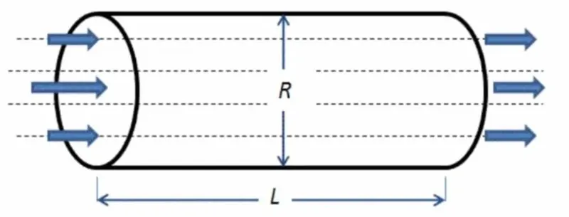
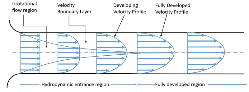
- The distance from the start of the flow to the point where the flow becomes fully developed.
- The hydrodynamic entrance region refers to the area of pipe where fluid entering a pipe develops a velocity profile due to viscous forces propagating from the interior walls of pipe. The flow in this region is non-uniform due to pipe friction, the length of the hydrodynamic region for laminar flow is given by
L = 0.0575 * Re * D
Blockmesh:
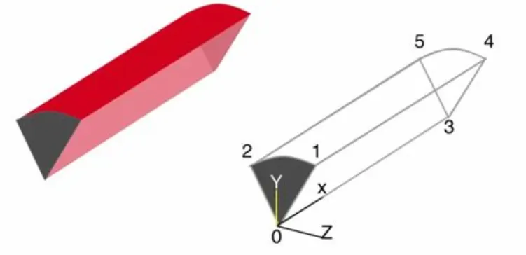
We need to create the block mesh in parafoam, for doing the whole section it will take more time and also it needs a high specification processor, so we can divide that whole section as a wedge and the flow becomes axi-symmetric. The cut angle can be fixed from 3 to 4 degrees.
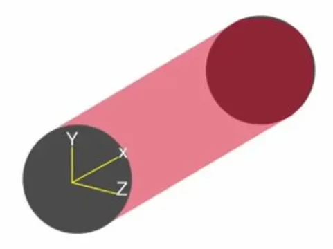
The wedge section of the pipe with 4 degree cut
vertices:
- inlet section (0 1 2 0)
- outlet section (3 5 4 3)
- front section (0 3 4 1)
- back section (0 2 5 3)
- top section (1 4 5 2)
- axis (0 3 3 0)
Shear stress and velocity distribution along the radius:
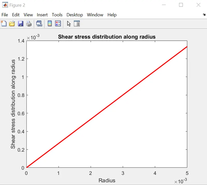
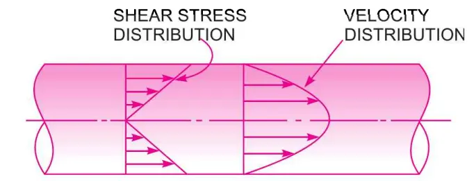
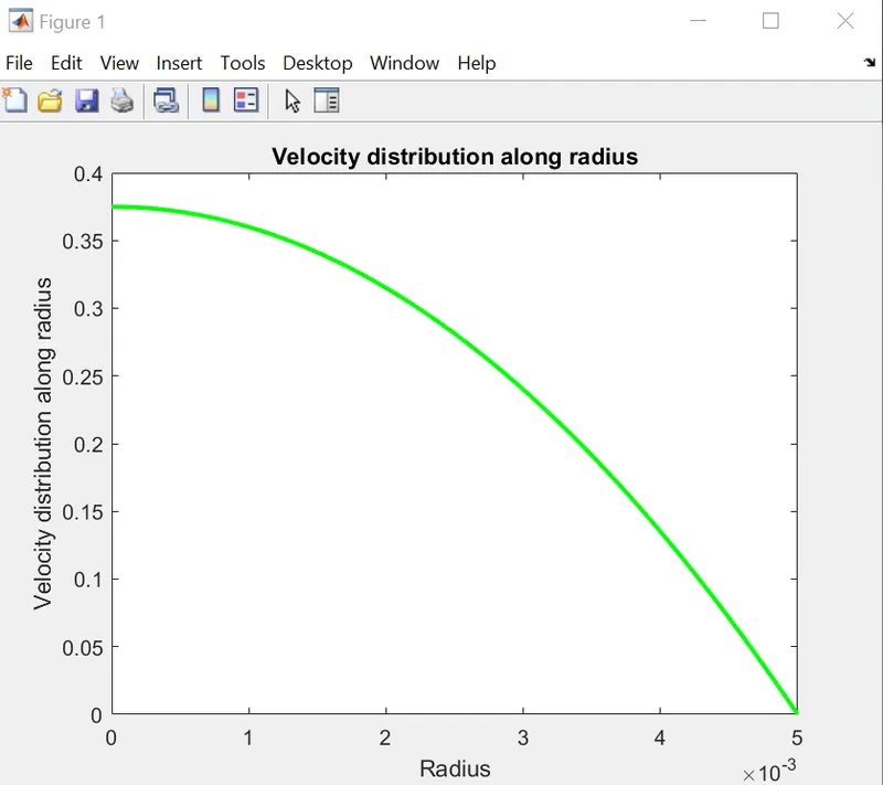
From the analytical results and from the below mentioned figure, we can say that shear stress is maximum at the wall of pipe, which means velocity is zero at the wall because of no slip condition and velocity is maximum is at the exact center section of pipe which means that shear stress is zero at that point.
PROCEDURE:
STEP-1:
First, we need to install the visual box and then we need to install the ubuntu in our system.
STEP-2:
we need to install the openFOAM software in ubuntu
STEP-3:
Now we need to open the terminal from the ubuntu desktop.
STEP-4:
The terminal is the command window where we can access to the folders, parafoam.
STEP-5:
cd - is the keyword which resembles "current directory"
ls - is the keyword which resembles "list" and it is used to list down the elements inside the folder.
In the terminal, we need to open the tutorials by using the command "cd $FOAM_TUTORIALS"
and followed by is explained in the picture.
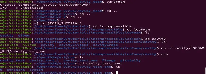
- From the picture we can see that after opening the tutorials we need to choose "cd incompressible", then "cd icoFoam"
- This icoFoam is used to calculate incompressible Navier Stoke's equation.
- From there we need to open the "cd cavity" and we need to copy this file in our directory so that we can run this by using the command "cp -r cavity/$FOAM_RUN/cavity_test".
- This cavity_test is the folder where we are going to save what we require.
- we will be having "0", "constant", "system" after listing down.
STEP-6:
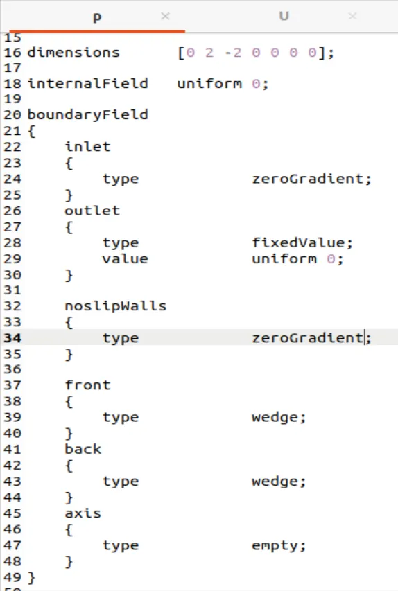
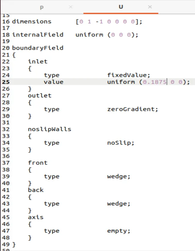
- By selecting "0" we will get two options one is "P" which is pressure and the other is "U", which is velocity. This has to be opened and it as to be edited according to our requirements and this can be done by using the command "gedit p" and "gedit u". "gedit" is a command which is used to open it because it is editable file.
- Now we need to give the values according to our requirements which is shown below.
STEP-7:
Similarly, we need to do for velocity file.
STEP-8:
- We need to edit the block mesh file or we need to create the file using MATLAB as follows,
- The code for creating file and this also contains analytical solution:
% % % % block mesh file for pipe flow
close all
clear
clc

% % initial conditions
% reynold's number
Re = 2100;
% density of water (kg/m^3)
rho = 997;
% dynamic viscosity of water (pa. s)
mu = 8.9 * 10^-4;
% kinematic viscosity of water (m^2/ s)
nu = mu/rho;
% diameter of pipe (m)
D = 0.01;
% radius of pipe (m)
R = D/2;
% area of pipe
A = pi * D^2;
% velocity (m/s)
V = (Re * mu)/(rho * D);
% gravity due to acelleration (m/s^2)
g  = 9.81;
% hydrodynamic length (m)
L_hd = 0.0575 * Re * D;
% total pipe length (m)
L_T = L_hd + 0.2925;
% wedge angle (THETA)
theta = 4;

% % % analytic calculations:
% % velocity calculations:
% average velocity
V_avg = V;
% maximum velocity
V_max = 2 * V_avg;
r = linspace(0,R,1000);
% variation of velocity along the radius of pipe
v_d = V_max * (1 - (r.^2/R^2));
L_V = linspace(0,L_T,1000);
% time
T_t = L_T/V_avg;

% discharge
Q = A * V_avg;

% Hagen Poiseuilles's Equation (head loss)
h_L = (32 * mu * V_avg * L_T)/(rho * g * D^2);

% h_L = (p1 - p2)/(rho * g)
% p1 - p2 = dp (pressure drop)
dp = h_L * rho * g;

% pressure gradient (P_G)
% -dp/dx = -dp/L = -(p1 - p2)/L = P_G
P_G = -dp/L_T;

% power required to overcome a head loss
P = (128 * mu * Q^2 * L_T)/(pi * D^4);

% %shear stress calculations:
% shear stress at boundary (wall shear stress)
ST_B = 8 * mu * V_avg;
% variation of shear stress along the radius of pipe
ST_V = (ST_B * r)/R;
% friction factor or Darcy's friction factor or Moody's friction factor
f_f = 64/Re;
% friction co-efficient or Fanning's co-efficient
f_c = f_f/4;

% Analytical plots
figure(1)
plot(r,v_d,'color','g','LineWidth',2)
title('Velocity distribution along radius')
xlabel('Radius')
ylabel('Velocity distribution along radius')
hold on

figure(2)
plot(r,ST_V,'color','r','LineWidth',2)
title('Shear stress distribution along radius')
xlabel('Radius')
ylabel('Shear stress distribution along radius')


% % mesh size
nx = 500;
ny = 50;
nz = 1;

% % to create the file
f1 = fopen('blockMeshDict', 'w');

% % file contents
fprintf(f1, 'FoamFile\n');
fprintf(f1, '{\n');
fprintf(f1, '     version      2.0;\n');
fprintf(f1, '     format       ascii;\n');
fprintf(f1, '     class        dictionary;\n');
fprintf(f1, '     object       blockMeshDict;\n');
fprintf(f1, '}\n\n\n');

fprintf(f1, 'convertTometers 1;\n\n');

fprintf(f1, 'vertices\n');
fprintf(f1, '(\n');
fprintf(f1, '     (0 0 0)\n');
%fprintf(f1, '     (0 R * cosd(theta/2) R * sind(theta/2))\n');
fprintf(f1, '     (%f\t   %f\t%f)\n',0, R * cosd(theta/2), R * sind(theta/2));

%fprintf(f1, '     (0 R * cosd(theta/2) -R * sind(theta/2),\n');
fprintf(f1, '     (%f\t   %f\t%f)\n',0, R * cosd(theta/2),-R * sind(theta/2));

%fprintf(f1, '     (L_T 0 0)\n');
fprintf(f1, '     (%f\t   %f\t%f)\n',L_T, 0, 0);

%fprintf(f1, '     (L_T R * cosd(theta/2) R * sind(theta/2))\n');
fprintf(f1, '     (%f\t   %f\t%f)\n',L_T, R * cosd(theta/2), R * sind(theta/2));

%fprintf(f1, '     (L_T R * cosd(theta/2) -R * sind(theta/2))\n');
fprintf(f1, '     (%f\t   %f\t%f)\n',L_T, R * cosd(theta/2),-R * sind(theta/2));
fprintf(f1, ');\n\n');

fprintf(f1, 'blocks\n');
fprintf(f1, '(\n');
%fprintf(f1,'      hex (0 3 5 2 0 3 4 1) (nx ny nz) simpleGrading (1 1 1)\n');
fprintf(f1, '      hex (%d %d %d %d %d %d %d %d) (%d %d %d) simpleGrading (1 1 1)\n',0, 3, 5, 2, 0, 3, 4, 1, nx, ny, nz);
fprintf(f1, ');\n\n');
fprintf(f1, 'edges\n');
fprintf(f1, '(\n');

%fprintf(f1, '      arc 1 2 (0 R 0)\n');
fprintf(f1,'       arc 1 2 (0 %f 0)\n',R);
%fprintf(f1, '      arc 4 5 (L_T R 0)\n');
fprintf(f1,'       arc 4 5 (%d %f 0)\n',L_T,R);
fprintf(f1, ');\n\n');

fprintf(f1, 'boundary\n');
fprintf(f1, '(\n');
fprintf(f1, '      inlet\n');
fprintf(f1, '      {\n');
fprintf(f1, '          type patch;\n');
fprintf(f1, '          faces\n');
fprintf(f1, '          (\n');
fprintf(f1, '              (0 1 2 0)\n');
fprintf(f1, '          );\n');
fprintf(f1, '      }\n');

fprintf(f1, '      outlet\n');
fprintf(f1, '      {\n');
fprintf(f1, '          type patch;\n');
fprintf(f1, '          faces\n');
fprintf(f1, '          (\n');
fprintf(f1, '              (3 5 4 3)\n');
fprintf(f1, '          );\n');

fprintf(f1, '      }\n');

fprintf(f1, '      frontAndBack\n');
fprintf(f1, '      {\n');
fprintf(f1, '          type wedge;\n');
fprintf(f1, '          faces\n');
fprintf(f1, '          (\n');
fprintf(f1, '              (0 1 2 0)\n');
fprintf(f1, '              (3 5 4 3)\n');
fprintf(f1, '          );\n');
fprintf(f1, '      }\n');

fprintf(f1, '      noslipWalls\n');
fprintf(f1, '      {\n');
fprintf(f1, '          type wall;\n');
fprintf(f1, '          faces\n');
fprintf(f1, '          (\n');
fprintf(f1, '              (2 1 4 5)\n');
fprintf(f1, '          );\n');
fprintf(f1, '      }\n');

fprintf(f1, '      axis\n');
fprintf(f1, '      {\n');
fprintf(f1, '          type empty;\n');
fprintf(f1, '          faces\n');
fprintf(f1, '          (\n');
fprintf(f1, '              (0 3 3 0)\n');
fprintf(f1, '          );\n');
fprintf(f1, '      }\n');

fprintf(f1, ');\n\n');

fprintf(f1, 'mergePatchPairs\n');
fprintf(f1, '(\n');
fprintf(f1, ');');
STEP-9:
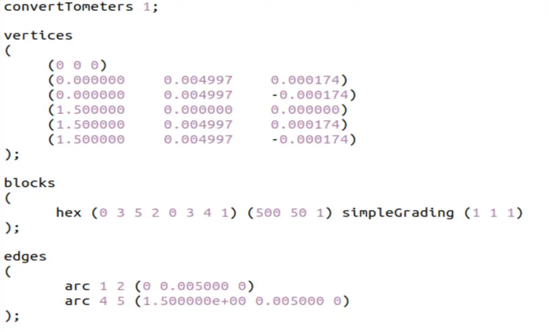
- Now we need to open "system" and there we need to select "blockMeshDict" and we need to replace file which has been created using MATLAB:
- "hex" is the keyword which resembles the type of mesh.
- Next to that is numbered faces of five geometry blocks.
- Next to that is to define number of cells along x, y and z axis.
- "simpleGrading" is the keyword which resembles grading factor and here in this case - 1 is "1".
- This part is to generate mesh.
- if there is wedge type problems, then we need to define edges also.
STEP-10:
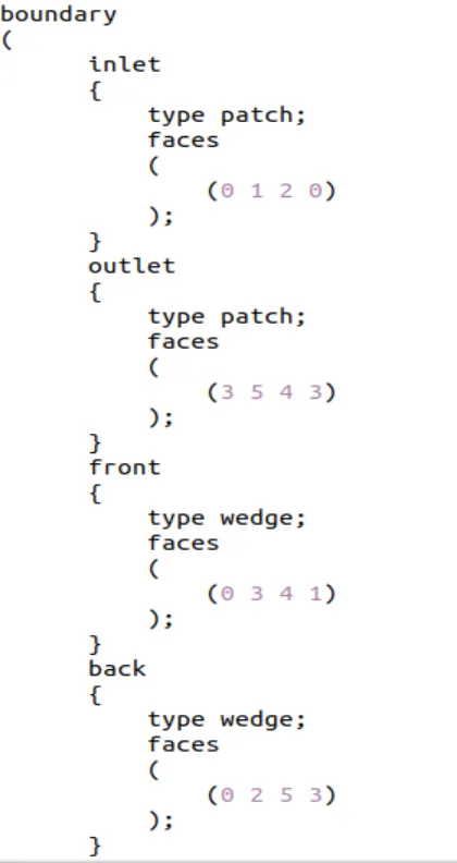
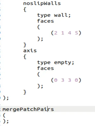
- In the blockMeshDict itself, we need to give the following details.
- We need to give boundary conditions such as "inlet", "outlet", "frontandback", "axis" and "noslipwalls"
STEP-11:
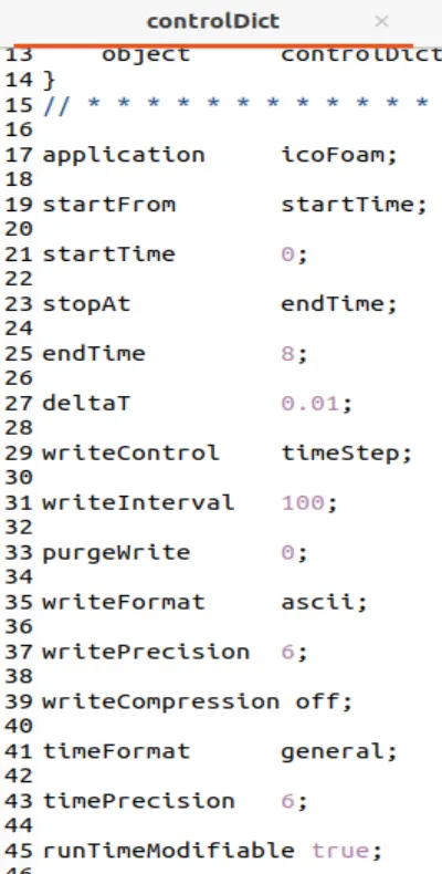
- Now we need to open "system" and there we need to select "controlDict" and we need to edit the following:
- We need to make sure that CFL number should be less than "0.5"
STEP-12:
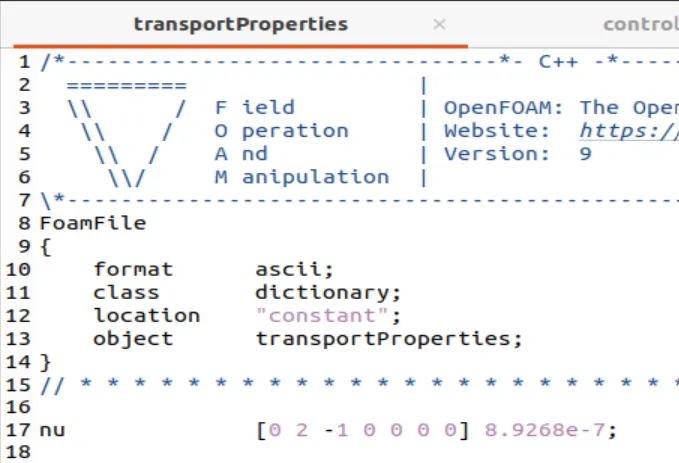
Now, we need to change the value of kinematic viscosity value in the "transportProperties"
STEP-13:
After completing all these settings, we need to save the things what we have done by pressing the "save" button which is on the right side top or "ctrl + s"
STEP-14:
Now we need to go back to the terminal and we need to give the command "blockMesh"
STEP-15:
Now the mesh generation is done. Then we need to solve the problem by using "icoFoam" solver.
STEP-16:
To view the simulation or simulated results, we need to open paraview and to that we need to give the command "paraFoam"
RESULTS AND OUTPUT:
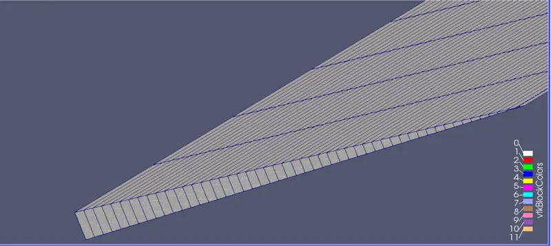
This is the meshed file of pipe wedge and which can be viewed in paraFoam which can be opened through terminal and we need to uncheck the fields so that we can able to see the meshed product.
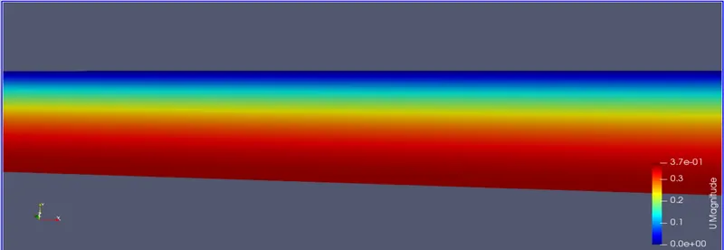
This shows the velocity distribution of the wedge and here we need to check the fields like velocity, so that we can able to see the product.
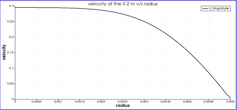
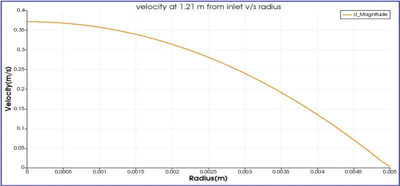
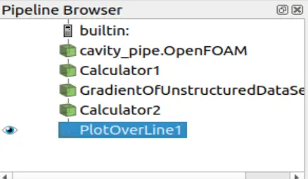
This plots are done by using the "plot over line" option which is available in the paraview and we need to select the fields what we want like pressure, density, temperature and velocity etc..
from analytic calculations,
Hydrodynamic length = 1.21 m
Total length = 1.5 m
1. Beginning of the flow:
2. Exactly at hydrodynamic length:
3. Exactly at the outlet:
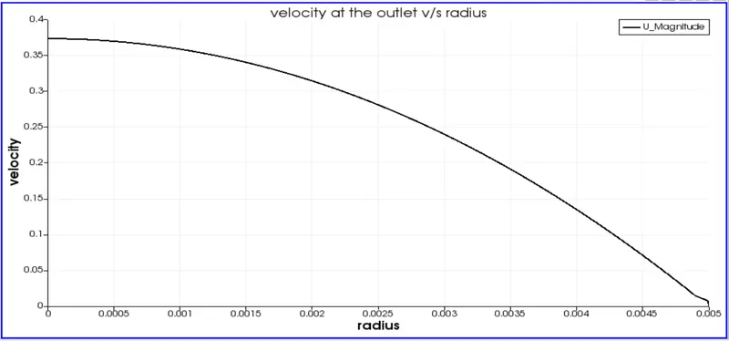
From the last three graphs we can say that graph at hydrodynamic length and and at total length are pretty much exact to each other because flow is not fully developed before hydrodynamic length
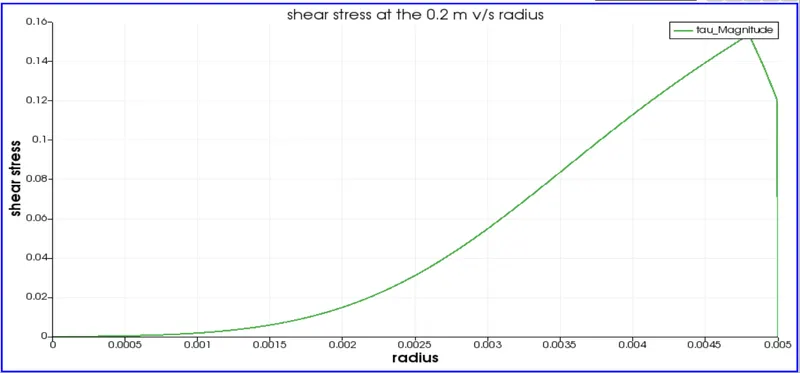
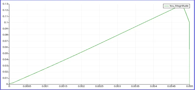
shear stress plots:
1. Beginning of the flow:
2. Exactly at hydrodynamic length:
3. Exactly at the outlet:
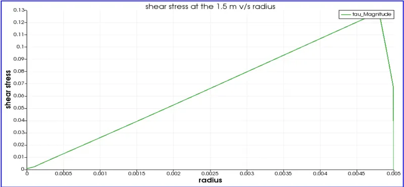
From the last three graphs we can say that graph at hydrodynamic length and and at total length are pretty much exact to each other because flow is not fully developed before hydrodynamic length.
ANALYTICAL PLOTS:
VELOCITY PLOT:
PRESSURE PLOT: